GPU Gems 3

GPU Gems 3 is now available for free online!

The CD content, including demos and content, is available on the web and for download.

You can also subscribe to our Developer News Feed to get notifications of new material on the site.

Chapter 40. Incremental Computation of the Gaussian

Ken Turkowski
Adobe Systems

We present an incremental method for computing the Gaussian at a sequence of regularly spaced points, with the cost of one vector multiplication per point. This technique can be used to implement image blurring by generating the Gaussian coefficients on the fly, avoiding an extra texture lookup into a table of precomputed coefficients.

40.1 Introduction and Related Work

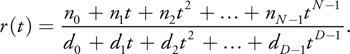
Filtering is a common operation performed on images and other kinds of data in order to smooth results or attenuate noise. Usually the filtering is linear and can be expressed as a convolution:

Equation 1

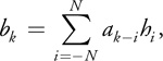
where a_i is an input sequence, b_i is an output sequence, and h_i is the kernel of the convolution.

One of the most popular filtering kernels is the Gaussian:

Equation 2

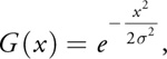
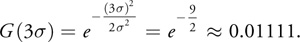
where is a parameter that controls its width. Figure 40-1 shows a graph of this function for = 1.

Figure 40-1 Gaussian with = 1.0

When used for images in 2D, this function is both separable and radially symmetric:

Equation 3

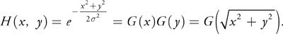
We can take advantage of this symmetry to considerably reduce the complexity of the computations.

Gaussian blurring has a lot of uses in computer graphics, image processing, and computer vision, and the performance can be enhanced by utilizing a GPU, because the GPU is well suited to image processing (Jargstorff 2004). The fragment shader for such a computation is shown in Listing 40-1.

In Listing 40-1,acc implements the summation in Equation 1, coeff is one of the coefficients h_i in the kernel of the convolution, texture2D() is the input sequence a_k _– _i , and gl_FragColor is one element of the output sequence b_k .

The coefficient computations involve some relatively expensive operations (an exponential and a division), as well as some cheaper multiplications. The expensive operations can dominate the computation time in the inner loop. An experienced practitioner can reduce the coefficient computations to

 coeff = exp(-u * u);

but still, there is the exponential computation on every pixel.

One approach to overcome these expensive computations would be to precompute the coefficients and look them up in a texture. However, there are already two other texture fetches in the inner loop, and we would prefer to do some computations while waiting for the memory requests to be fulfilled.

Example 40-1.

    uniform sampler2D inImg;  // source image    uniform float     sigma;  // Gaussian sigma    uniform float     norm;   // normalization, e.g. 1/(sqrt(2*PI)*sigma)    uniform vec2      dir;    // horiz=(1.0, 0.0), vert=(0.0, 1.0)    uniform int       support; // int(sigma * 3.0) truncation    void main() {   vec2 loc = gl_FragCoord.xy;    // center pixel cooordinate    vec4 acc;                      // accumulator   acc = texture2D(inImg, loc);   // accumulate center pixel    for (i = 1; i <= support; i++) {     float coeff = exp(-0.5 * float(i) * float(i) / (sigma * sigma));     acc += (texture2D(inImg, loc - float(i) * dir)) * coeff; // L     acc += (texture2D(inImg, loc + float(i) * dir)) * coeff; // R   }   acc *= norm;            // normalize for unity gain   gl_fragColor = acc; }

Another approach would be to compute the Gaussian using one of several polynomial or rational polynomial approximations that are chosen based on the range of the argument. However, range comparisons are inefficient on a GPU, and the table of polynomial coefficients would most likely need to be stored in a texture, so this is less advantageous than the previous approach.

Our approach is to compute the coefficients on the fly, taking advantage of the coherence between adjacent samples to perform the computations incrementally with a small number of simple instructions. The technique is analogous to polynomial forward differencing, so we take a moment to describe that technique first.

40.2 Polynomial Forward Differencing

Suppose we wish to evaluate a polynomial

Equation 4

M times at regular intervals starting at t ₀, that is,

{t₀, t₀ + + 2, ..., t₀ + (M-1)}.

We hope to use the coherence between successive values to decrease the amount of computation at each point. We know that, for a linear (that is, second order) polynomial L(t) = at + b, the difference between successive values is constant:

Equation 5

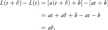
which results in the following forward-differencing algorithm to compute a sequence of linear function values at regular intervals dt, starting at a point t ₀:

 p0 = a * t0 + b; p1 = a * dt; for (i = 0; i < LENGTH; i++) {   DoSomethingWithTheFunctionValue(p0);   p0 += p1; }

We extend this algorithm to an N-order polynomial by taking higher-order differences and maintaining them in N variables whose values at iteration i are denoted as

These N variables are initialized as the repeated differences of the polynomial evaluated at successive points:

Equation 6

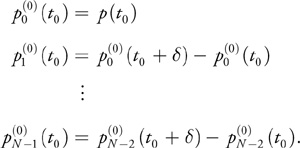
That is, we first take differences of the polynomial evaluated at regular intervals, and then we take differences of those differences, and so on. It should come as no surprise that the Nth difference is zero for an Nth-order polynomial, because the differences are related to derivatives, and the Nth derivative of an Nth-order polynomial is zero. Moreover, the (N - 1)th difference (and derivative) is constant.

At each iteration i, the N state variables are updated by incrementing

The value of the polynomial at t ₀ + i is then given by .

For example, to incrementally generate a cubic polynomial

Equation 7

we initialize the forward differences as such:

Equation 8

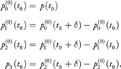
where is the value of the polynomial at the initial point, and are the first and second differences at the initial point, and p ₃ is the constant second difference. Note that we have dropped the iteration superscript on p ₃ because it is constant.

To evaluate the polynomial at t ₀ + by the method of forward differences, we increment p ₀ by p ₁, p ₁ by p ₂, and p ₂ by p ₃:

Equation 9

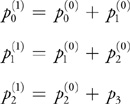
and the value is given by .

Similarly, the value of the polynomial at t ₀ + 2 is computed from the previous forward differences:

Equation 10

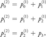
and so on. Note that in the case of a cubic polynomial, we can use a single state vector to store the forward differences. Utilizing the powerful expressive capabilities of GLSL, we can implement the state update in one instruction:

 p.xyz += p.yzw;

where we have initialized the forward-difference vector as follows:

 p = f(vec4(t, t+d, t+2*d, t+3*d)); p.yzw -= p.xyz; p.zw  -= p.yz; p.w   -= p.z;

Note that this method can be used to compute arbitrary functions, not just polynomials. Forward-differencing is especially useful for rendering in 2D and 3D graphics using scan-conversion techniques for lines and polygons (Foley et al. 1990). Adaptive forward differencing was developed in a series of papers (Lien et al. 1987, Shantz and Chang 1988, and Chang et al. 1989) for evaluating and shading cubic and NURBS curves and surfaces in floating-point and fixed-point arithmetic. Klassen (1991a) uses adaptive forward differencing to draw antialiased cubic spline curves. Turkowski (2002) renders cubic and spherical panoramas in real time using forward differencing of piecewise polynomials adaptively approximating transcendental functions.

Our initialization method corresponds to the Taylor series approximation. More accurate approximations over the desired domain can be achieved by using other methods of polynomial approximation, such as Lagrangian interpolation or Chebyshev approximation (Ralston and Rabinowitz 1978).

40.3 The Incremental Gaussian Algorithm

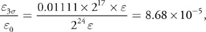
When we apply the forward-differencing technique to the Gaussian, we get poor results, as shown in Figure 40-2.

Figure 40-2 Gaussian Approximated by a Polynomial

The orange curve in Figure 40-2 is the Taylor series approximation at 0, and the green curve is a polynomial fit to the points {0.0, 1.0, 2.0}. The black curve is the Gaussian. The fundamental problem is that polynomials get larger when their arguments do, whereas the Gaussian gets smaller.

The typical numerical analysis approach is to instead use a rational polynomial of the form

Equation 11

We can also use forward differencing to compute the numerator and the denominator separately, but we still have to divide them at each pixel. This algorithm does indeed produce a better approximation and has the desired asymptotic behavior. This is a good technique for approximating a wide class of functions, but we can take advantage of the exponential nature of the Gaussian to yield a method that is simpler and faster. It turns out that we have such an algorithm that shares the simplicity of forward differencing if we replace differences by quotients.

Given the Gaussian

Equation 12

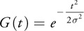
we evaluate the quotient of successive values

Equation 13

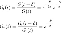
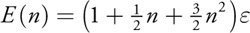
and we find that the second quotient is constant, whereas the first quotient is exponential, as illustrated in Figure 40-3.

Figure 40-3 Gaussian with First and Second Quotients

The next quotient would yield another constant: 1. These properties have a nice analogy to those of forward differencing, where quotients take the place of differences, and a quotient of 1 takes the place of a difference of 0.

Note that there are two factors in the first quotient: one is related purely to the sampling spacing , and the other is an attenuation from t = 0. In fact, when we set t = 0, we get

Equation 14

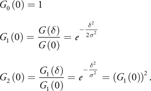
Only one exponential evaluation is needed to generate any number of regularly spaced samples starting at zero. The entire Gaussian is characterized by one attenuation factor, as shown in Listing 40-2.

Example 40-2.

 #ifdef USE_SCALAR_INSTRUCTIONS // suitable for scalar GPUs float g0, g1, g2; g0 = 1.0 / (sqrt(2.0 * PI) * sigma); g1 = exp(-0.5 * delta * delta / (sigma * sigma)); g2 = g1 * g1; for (i = 0; i < N; i++) {   MultiplySomethingByTheGaussianCoefficient(g0);   g0 *= g1;   g1 *= g2; } #else // especially for vector architectures float3 g; g.x = 1.0 / (sqrt(2.0 * PI) * sigma); g.y = exp(-0.5 * delta * delta / (sigma * sigma)); g.z = g.y * g.y; for (i = 0; i < N; i++) {   MultiplySomethingByTheGaussianCoefficient(g.x);   g.xy *= g.yz; } #endif // USE_VECTOR_INSTRUCTIONS

The Gaussian coefficients are generated with just one vector multiplication per sample. A vector multiplication is one of the fastest instructions on the GPU.

40.4 Error Analysis

The incremental Gaussian algorithm is exact with exact arithmetic. In this section, we perform a worst-case error analysis, taking into account (1) errors in the initial coefficient values, which are due to representation in single-precision IEEE floating-point (that is, a(1 + )) and (2) error that is due to floating-point multiplication (ab(1 + )). Then we determine how the error grows with each iteration.

Let the initial relative error of any of the forward quotient coefficients be a stochastic variable so that its floating-point representation is

Equation 15

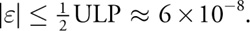
instead of a, because it is approximated in a finite floating-point representation. For single-precision IEEE floating-point, for example,

The product of two finite-precision numbers c and d is

Equation 16

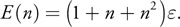
instead of cd because the product will be truncated to the word length. Putting this together, we find that the relative error of the product of two approximate variables a and b is

Equation 17

Thus, the errors accumulate. As is traditional with error analysis, we drop the higherorder terms in , because they are much less significant.

The relative error for the coefficients is shown in Table 40-1, computed simply by executing the incremental Gaussian algorithm with the error accumulation just given. Here, we do two exponential computations: one for the first-order quotient g ₁ and one for the second-order quotient g ₂, to maximize the precision.

Table 40-1. Growth in Coefficient Error

Iteration	g ₀ Error	g ₁ Error	g ₂ Error
0
1	3	3
2	7	5
3	13	7
4	21	9
·	·	·	·
·	·	·	·
·	·	·	·

The error in g ₁ increases linearly, because it is incremented by the constant g ₂ every iteration. The error in g ₀ also accumulates the error in g ₁, so it grows quadratically. The error for g ₀ can then be expressed as a polynomial function of n:

Equation 18

If the initial error is 1/2 of the least significant bit of a single-precision floating-point number and we wish the coefficients to have a relative error of 1/256, then the parenthesized quantity in the Equation 18 should be less than 2¹⁷. This suggests n 361.

Typically, however, practitioners truncate the Gaussian at 3, where

Equation 19

The error in the last evaluation (at 3), relative to the central coefficient is still only

Equation 20

when we compute it with 361 forward products. If we are willing to have a maximum error of 1/256 relative to the central coefficient (as opposed to the error relative to the fringe coefficient), then we can go up to 3,435 samples. When these coefficients are used to implement a convolution kernel, this is the kind of accuracy that we need.

We have a different situation if we choose to do only one exponential computation for the first quotient and compute the second difference from the first. In this case the error in the second quotient is doubled, as shown in Table 40-2.

Table 40-2. Growth in Coefficient Error When g ₂ Is Computed from g ₁

Iteration	g ₀ Error	g ₁ Error	g ₂ Error
0			2
1	3	4	2
2	8	7	2
3	16	10	2
4	27	13	2
·	·	·	·
·	·	·	·
·	·	·	·

The error for g ₀ in this scenario is

Equation 21

with the maximum number of iterations for 8-bit accuracy 295 or 2,804, depending on whether the relative accuracy desired is relative to the fringe or the central coefficients, respectively.

For image-blurring applications, the fringe error relative to the central coefficient is of primary concern. Even when we compute g ₂ from g ₁, the limitation of 3 2804, or s 934 is not restrictive (because applications with s > 100 are rare), so it suffices to compute only the g ₁ coefficient as an exponential, and g ₂ as its square.

40.5 Performance

Processor performance has increased substantially over the past decade, so that arithmetic logic unit (ALU) operations are executed faster than accessing memory, by one to three orders of magnitude. As a result, algorithms on modern computer architectures benefit from replacing table lookups with relatively simple computations, especially when the tables are relatively large.

The incremental computation algorithm is noticeably faster on the GPU and CPU than looking up coefficients in a table. While GPU performance highly depends on the capabilities of the hardware, the GPU vendor, the driver version, and the operating system version, we can conservatively say that the technique yields at least a 15 percent performance improvement.

Another aspect of performance is whether a particular blur filter can fit on the GPU. The incremental Gaussian blur algorithm may appear to be small, but the GPU driver will increase the number of instructions dramatically, under certain circumstances. In particular, some GPUs do not have any looping primitives, so the driver will automatically unroll the loop. The maximum loop size (that is, the Gaussian radius) is then limited by the number of ALU instructions or texture lookup instructions. This algorithm will then reduce the number of texture lookups to increase the maximum blur radius.

Graphics hardware architecture is constantly evolving. While texture access is relatively slow compared to arithmetic computations, some newer hardware (such as the GeForce 8800 Series) incorporates up to 16 constant buffers of 16K floats each, with the same access time as a register. The incremental Gaussian algorithm may not yield any higher performance than table lookup using such constant buffers, but it may not yield lower performance either. The incremental Gaussian algorithm has the advantage that it can be deployed successfully on a wide variety of platforms.

40.6 Conclusion

We have presented a very simple technique to evaluate the Gaussian at regularly spaced points. It is not an approximation, and it has the simplicity of polynomial forward differencing, so that only one vector instruction is needed for a coefficient update at each point on a GPU.

The method of forward quotients can accelerate the computation of any function that is the exponential of a polynomial. Modern computers can perform multiplications as fast as additions, so the technique is as powerful as forward differencing. This method opens up incremental computations to a new class of functions.

40.7 References

Chang, Sheue-Ling, Michael Shantz, and Robert Rocchetti. 1989. "Rendering Cubic Curves and Surfaces with Integer Adaptive Forward Differencing." In Computer Graphics (Proceedings of SIGGRAPH 89), pp. 157–166.

Foley, James D., Andries van Dam, Steven K. Feiner, and John F. Hughes. 1990. Computer Graphics: Principles and Practice. Addison-Wesley.

Jargstorff, F. 2004. "A Framework for Image Processing." In GPU Gems, edited by Randima Fernando, pp. 445–467. Addison-Wesley.

Klassen, R. Victor. 1991a. "Drawing Antialiased Cubic Spline Curves." ACM Transactions on Graphics 10(1), pp. 92–108.

Klassen, R. Victor. 1991b. "Integer Forward Differencing of Cubic Polynomials: Analysis and Algorithms." ACM Transactions on Graphics 10(2), pp. 152–181.

Lien, Sheue-Ling, Michael Shantz, and Vaughan Pratt. 1987. "Adaptive Forward Differencing for Rendering Curves and Surfaces." Computer Graphics (Proceedings of SIGGRAPH 87), pp. 111–118.

Ralston, Anthony, and Philip Rabinowitz. 1978. A First Course in Numerical Analysis, 2nd ed. McGraw-Hill.

Shantz, Michael, and Sheue-Ling Chang 1988. "Rendering Trimmed NURBS with Adaptive Forward Differencing." Computer Graphics (Proceedings of SIGGRAPH 88), pp. 189–198.

Turkowski, Ken. 2002. "Scanline-Order Image Warping Using Error-Controlled Adaptive Piecewise Polynomial Approximation." Available online at http://www.worldserver.com/turk/computergraphics/AdaptPolyFwdDiff.pdf.

I would like to thank Nathan Carr for encouraging me to write a chapter on this algorithm, and Paul McJones for suggesting a contribution to GPU Gems. Gavin Miller, Frank Jargstorff and Andreea Berfield provided valuable feedback for improving this paper. I would like to thank Frank Jargstorff for his evaluation of performance on the GPU.