GPU Gems 3

GPU Gems 3 is now available for free online!

The CD content, including demos and content, is available on the web and for download.

You can also subscribe to our Developer News Feed to get notifications of new material on the site.

Chapter 33. LCP Algorithms for Collision Detection Using CUDA

Peter Kipfer
Havok

An environment that behaves correctly physically is central to the immersive experience of a computer game. In some games, the player is even forced to interact with objects in the scene in a way that is critical to succeeding in the game level. Physics simulation therefore has become a mission-critical software component for game developers. The main challenge for developing game physics is minimizing the processor usage of the simulation, because the available resources are already heavily loaded with game AI, asset handling, animation, and graphics preprocessing. What complicates the situation further is that all these components depend on a consistent representation of the physics world and heavily depend on being able to query information from it.

In this chapter, we use CUDA to accelerate convex collision detection, and we study a parallel implementation of Lemke's algorithm (also called the complementary pivot algorithm) (Lemke 1965) for the linear complementarity problem (LCP). Important LCP applications are linear and quadratic programming, two-person games, boundaryvalue problems, and the determination of the convex hull of points in a plane. A parallel version of the algorithm was first proposed by Thompson (1987) with near-linear speedup for low numbers of processors.

33.1 Parallel Processing

A natural approach to speed up the calculations needed for a particular simulation is to split up the work to multiple processors. Modern computer systems have several programmable units. The main CPU nowadays features multiple execution cores, and specialized parallel algorithms on graphics hardware have become important building blocks for highly responsive simulations.

There is a huge amount of literature on parallel computing. CUDA provides an environment that has many of the standard parallelization features used on multi-CPU computers. It is thus worth investigating existing parallel algorithms for their suitability to run efficiently on the current GPU generation. This will allow us to perhaps dynamically shift workload between processing units, which is still tedious with previous-generation GPUs because of restricted functionality. NVIDIA's current generation of GPUs has changed from a rather rigid four-component vector processor to a scalar architecture featuring several SIMD multiprocessors. The GPU still is very specific in terms of its memory access patterns. While parallel CPU threads usually communicate over main memory, the current generation of GPUs move the shared memory block nearer to the ALUs. This has implications for the communication and synchronization granularity necessary for an efficient algorithm. Existing parallel algorithms therefore must be adapted to this change.

In this chapter, we examine the opportunities presented by the new CUDA programming environment for advanced solver techniques in the context of physics simulation. The involved numerics have not been a major problem on the previous GPU generation, but the missing flexibility with respect to memory addressing and limited output bandwidth have prevented many algorithms from running efficiently on the GPU. The CUDA environment solves these problems and provides additional features vital for concurrent processing: thread synchronization as well as thread-shared and thread-local storage. These enhancements allow us to bring a class of algorithms to the GPU that would have been impossible to implement before: multithreaded cooperative parallel programs.

33.2 The Physics Pipeline

The processing pipeline for rigid body physics is usually split into three major blocks: broad phase, narrow phase, and resolution phase. Each phase has a specific task to solve and needs a different view of the participating objects to be simulated.

The broad phase does a coarse and quick check to determine which of the objects can experience a collision at all. It produces a pair list of potential collision partners. For fast comparisons, very simple data structures are used, such as bounding spheres or axis-aligned bounding boxes, as shown in Figure 33-1a. The general understanding, furthermore, is that most of the time, the motion of the objects per simulated time step is small compared to their bounding box size. Algorithms that can exploit this coherence are readily available (such as sweep-and-prune).

Figure 33-1 The Three Main Phases of the Processing Pipeline for Rigid Body Physics

The narrow phase obtains the collision pair list and for every pair, using their actual geometry, it checks whether the two partners are colliding. This phase can get arbitrarily complex, so in the context of real-time physics simulation, the participating colliding shapes are usually restricted to being convex. For nonconvex shapes, only the convex hull will then be used for collision detection. In most cases this is good enough—for example if the concavities are small or constitute object parts where you don't want a game character to go anyway, such as the exhaust pipes of a spacecraft or other irrelevant places. To improve collision quality and performance, we can decompose big or concave objects into convex pieces. A game object therefore might hold a simplified collision geometry that is different from the one displayed. In this chapter we investigate a narrow-phase algorithm for determining the distance between two convex objects. For the two objects in Figure 33-1b, the contact point marked with the yellow star is detected, and its location is calculated and stored with the collision pair.

Finally, the resolution phase computes forces according to the result of the narrow phase for pushing penetrating objects apart at every contact point. Because an object might collide with several others, appropriate handling of multiple contacts has to be done.

The resulting contact forces and velocities, shown as green arrows in Figure 33-1c, together with body properties (such as inertias) are then inserted into the formulas for rigid body motion, and the objects are integrated in time.

33.3 Determining Contact Points

The problem of determining contact points is covered in an immense amount of literature. The algorithms can be divided into two main groups. First, finding contact points from time t ₀ to t ₁ can be viewed as a single, continuous function of time. Here, the basic problem is to determine the time of first contact. Alternatively, the problem can be considered discretely, at a sequence of time increments t ₀ < t ₀ + ₁ < t ₀ + ₂ < . . . < t ₀ + _n < t ₁. Here, given the positions of bodies at time t ₀ + _i , the bodies have to be tested for interpenetration. Figure 33-2 compares the two approaches. The continuous approach on the bottom can consider, for example, the intersection of the swept volume of the object from time t ₀ to t ₁ with other objects in the scene analytically to solve for ₀, the time of first contact. The discrete approach in this case would simply check for overlap at the three positions.

Figure 33-2 Comparison of the Discrete and Continuous Collision Detection Approaches

33.3.1 Continuum Methods

The first approach assumes a specified motion of bodies over some time interval. Algorithms for determining the first collision between rigid polyhedral objects with constant angular velocity have been described in the literature using roots of (low-order) polynomials. However, for the general case of arbitrary trajectories of rigid convex polyhedra, no closed-form solution for the time of first contact exists, and iterative numerical methods are used to determine it.

Because the continuum methods assume a specified motion path of the bodies over time, they cannot solve the contact-point problem globally, because such a path is exactly what the simulator is trying to compute. Used over appropriately short time intervals, they however guarantee that collisions between objects are not missed, as for example happens with the discrete method in Figure 33-2. These continuum methods, especially those based on interval analysis, are complicated to implement and are not currently as fast as the discrete methods.

33.3.2 Discrete Methods (Coherence Based)

The second approach involves the geometric analysis of bodies at a point in time. The goal is to solve a single, static instance of the problem with optimal asymptotic time complexity. The most prominent algorithm here is the Gilbert-Johnson-Keerthi distance algorithm, which computes the minimum distance between convex polyhedra with n vertices. The algorithm has a complexity between O(n) and O(n log n), depending on stability optimizations present. For the problem of determining disjointness of two convex polyhedra with n vertices (without regard to the distance between them), a simpler O(n) algorithm based on linear programming is available.

Unfortunately, the small asymptotic time complexity comes at the price of large runtime constants. However, the involved algorithms offer good potential for parallel processing. In this chapter, we develop such a parallel solution using CUDA.

33.3.3 Resolving Contact Points

After determining when and where objects contact each other, we need to enforce noninterpenetration constraints. There are two basic approaches for preventing interpenetration between contacting objects without friction. The first approach, also called the penalty method, models contacts by placing a damped spring at each contact point, between the two contacting bodies. Interpenetration is allowed between the bodies at a contact point, but as the amount of interpenetration increases at a contact point, a repulsive restoring, or penalty, force acts between the objects, pushing them apart. The penalty method is a very attractive model, because it is extremely simple to implement and numerically simple. In particular, exploiting parallelism for GPU implementations on previous-generation hardware is rather straightforward.

The second approach computes constraint forces that are designed to exactly cancel any external accelerations that would result in interpenetration. This method requires solving nonlinear systems of equations. The CUDA solver developed in this chapter can be used for computing such forces. It results in simulations where interpenetration is completely eliminated (within numerical tolerances).

33.4 Mathematical Optimization

33.4.1 Linear Programming

Let's take a look at a simple optimization problem. We want to know whether or not two 2D polygons intersect. Consider the two triangles from Ericson 2005 given in Figure 33-3. The interior of each triangle can be described as an intersection of the half-spaces defined by its edges.

Figure 33-3 Two Intersecting Triangles

Triangle A is described by these three half-space equations:

-u + v -1, -u - 4v -1, 4u + v 19

and triangle B is given as the following:

- 4u + v 0, u - 4v 0, u + v 5.

In matrix notation this gives inequality constraints Ax b and an objective function c ^T x to be maximized, where c is a vector of constants. Because any point that is common to both triangles is a witness of their collision, the objective function can be chosen arbitrarily, for example c = (1, 0, . . ., 0). To solve the system for a maximum of x using the simplex algorithm, we introduce slack variables s to turn the inequalities into equalities—that is, for the inequality in every component i of the vector x : A_i x_i b_i , we write A_ix_i + s_i = b_i . The slack variable s thus takes the difference to fulfill the equality. For this simple case, direct solution methods or even exhaustive testing of the halfspaces might be faster, but the presented idea is general enough to support arbitrary convex polyhedra. This is important for a physics engine, to allow queries between any objects in the simulation.

The given linear programming problem answers the question whether two objects overlap or not. So in case an overlap is detected, the physics simulation is actually in an invalid state with penetrating rigid bodies. This has to be avoided, and therefore we'd like to perform a distance query between separated objects. This, however, cannot be answered using the current process.

33.4.2 The Linear Complementarity Problem

One important observation in linear programming is that for every maximization problem, there is a dual minimization problem. The strong duality principle states that you can optimize either the original or the dual problem to arrive at the same value. The consequence of this is that the slack variables of the original and the dual problems are related (complementary slackness). The vector of slack variables of the original problem is s = b - Ax 0; the vector of the dual problem is u = A ^T y - c. Therefore we can conclude that we have found an optimal solution only if either x_j = 0 or u_j = 0 or either y_i = 0 or s_i = 0. The idea now is to combine both the original and the dual problems into what is called a complementarity problem.

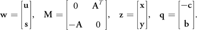
In linear algebra, the linear complementarity problem is formulated as follows:

Equation 1

where M is a real n-dimensional matrix and q is a given vector in ⁿ . Because of the last restriction, either w_i = 0 or z_i = 0 for i = 1, . . ., n, hence the name "complementarity problem." Apart from the trivial solution z = 0, w = q, if M is a P-matrix, it can be shown that this system has either a unique optimal solution or is unsolvable. In mathematics, a P-matrix is a square matrix with every principal minor greater than zero. Using the complementary slackness, our linear optimization problem from Equation 1 can be written as an LCP:

Note how this implicitly optimizes the objective function, because the solution vector of the LCP is the optimal feasible vector of the original and the dual problems.

33.4.3 Quadratic Programming

For our purpose of determining the distance between two objects, the objective function contains a quadratic term in addition to the linear term—that is, f(x) = x ^T Sx - c ^T x, and we are therefore faced with a problem of quadratic programming. The constraints are still linear, g(x) = (Ax - b, -x) 0, so we can use the LCP representation to solve it using the Karush-Kuhn-Tucker (KKT) conditions: Recall from calculus that a differentiable function has extreme points where its first derivative is zero. The KKT conditions state the same for the optimization problem as follows:

Equation 2

where f (x) is the gradient of f and G is the derivative matrix of g. The feasible points of this equation system are the local minima of the optimization problem. If we now additionally restrict f to be a convex function, we have a convex quadratic programming problem, and the following convenient statements are true:

If a local minimum exists, then it is a global minimum.
The set of all (global) minima is convex.
If the function f is strictly convex, then there exists at most one minimum.

In the context of physics simulation, for the two convex quadratic programming applications of calculating the distance between two convex polyhedra and for solving for impulse forces for resting contacts, we are therefore guaranteed to find the global optimal solution if it exists.

33.5 The Convex Distance Calculation

Let's do a simple example and determine the squared distance between two triangles in 2D. If P ₀ is a point inside the first triangle and P ₁ is a point inside the second triangle, then we'd like to minimize the squared distance

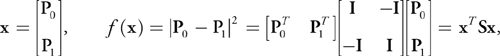
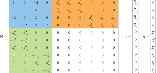
where I is the 2D identity matrix. The matrix S therefore has diagonal blocks I and offdiagonal blocks -I, and its eigenvalues are = 0 and = 2, hence it is symmetric and positive-semidefinite and the LCP will either be unsolvable or return an optimal solution. The constraints of the problem are that the two points must be inside the triangles. We can express that using the half-space inequalities from the preceding linear programming example. The minimum obviously is then reached for points lying on the triangle edges. Using the definition from Equation 2, we set up the LCP problem shown in Equation 3.

The blue part of Equation 3 is the matrix 2S, the orange part is A ^T , and the green part is -A. Note that the solution z vector conveniently contains the two optimal contact points in its first four components. This matrix is expanded easily for higher dimensions and more constraints, making it easy to formulate a canonical system for solving for the distance between convex polyhedra in 3D. Also note that the participating polyhedra do not need to have the same number of faces nor do they need the faces to be triangular.

Equation 3 An Example LCP Problem

33.5.1 Lemke's Algorithm for Solving the LCP

Lemke's algorithm operates on an equivalent, augmented linear complementarity problem by adding an artificial variable z ₀:

Equation 4

A basic feasible point, which is a basic vector such that (w, w ₀, z, z ₀) 0, is immediately available. A solution (z, z ₀) (w, w ₀) is said to be almost complementary if it is feasible and z _i w _i = 0 for all i = 0, . . ., n except for at most one i. The algorithm now moves (at every nondegenerate step) from a basic vector for Equation 4 to a new one maintaining the property of almost complementarity between (z, z ₀) and (w, w ₀) until either a complementary basic feasible solution for Equation 4 is obtained or an unbounded ray is detected. In every step, a Gauss-Jordan-elimination pivoting operation is performed. The current basis is modified by bringing into the basis a new variable and dropping a variable from the current set. The new entering variable is uniquely determined by the complementary pivot rule (that is, pick the variable that is complementary to the variable that just left the basis). The variable to drop from the basis is determined by the minimum ratio test of the simplex algorithm.

We refer the reader to Murty 1988 for details and definitions as well as the convergence of the algorithm. The algorithm features a method for preventing pivoting cycles and always terminates in a finite number of steps for important classes of matrices M, such as positive semidefinite matrices and matrices with positive entries.

33.6 The Parallel LCP Solution Using CUDA

From the example in Equation 3 and Lemke's algorithm for parallelization, it immediately becomes clear that we can parallelize the pivoting algorithm for the matrix. In particular, we can update the columns of the matrix concurrently, provided that the pivot column is available. Following Thompson 1987, we partition the matrix M among CUDA threads by rows; that is, each thread is responsible for one of the rows of the matrix M. The right-hand-side vector q is available to all threads, and a list of current basic and nonbasic variables is maintained.

At the beginning of each iteration, the pivot column is determined by the complementary pivot rule. Each thread independently computes the pivot row using the minimum ratio test and updates its portion of the matrix. This can be done in parallel, because each thread has an updated copy of the right-hand-side vector q and can compute the current pivot column. For optimization, the pivot column is computed in threadshared memory of the multiprocessor.

33.6.1 Implementation of the Solver

The CUDA LCP solver has three main tasks:

Select the pivot element
Solve for the selected equation variable
Check for termination

A solution has to be computed for every collision pair. Computing each solution is independent of each other. We therefore map the collision pair list to CUDA's compute grid. Each block has as many threads as there are equations in the LCP. Because the threads can communicate partial results, solving the LCP equations can be done in a cooperative manner by the threads. Figure 33-4 gives an overview of the processing.

Figure 33-4 CUDA Processing of the LCP Problem

The number of equations needed to set up the specific LCP problem for convex distance calculation depends on the dimension of the domain and the number of half-spaces. We get one equation per dimension of each of the two points' distances and one for each participating half-space constraint. For calculating the distance between two triangles in 2D, this amounts to 2 x 2 + 3 + 3 = 10 equations (see Equation 3). If arbitrary polygons are participating, obviously the number of constraints varies. To run the entire pair list as a CUDA grid, however, the number of threads per block must be the same for all blocks. We handle this by storing the number of equations per block and let excessive threads idle. This is more efficient than calling the kernel for each block separately, and it can be programmed very easily because each thread knows its cardinality. Note that this would have been very difficult to solve on previous GPU architectures. The number of threads needed for this approach quickly reaches quite large numbers. This has been a problem for past implementations on multiprocessor machines. For CUDA, however, this approach is ideal, because the GPU is optimized for handling high thread counts. To solve for the 3D distance between two convex objects with 60 faces each, we need 129 threads. This is a reasonable number for a CUDA kernel. Object descriptions easily get even more complicated when dealing with convex decompositions of concave objects.

The entire grid can therefore be covered by the same kernel. This is a very powerful feature, and we take advantage of that by implementing the control loop over the three steps previously mentioned also in the kernel. We therefore do not need to read back any intermediate status. When the kernel returns, each of the blocks will have either computed a solution or flagged itself as unsolvable. The implementation of the second step takes care of producing a contiguous list of results (see Figures 33-5 and 33-6), which allows us to download it efficiently in one batch.

Figure 33-5 The Pivot Selection Algorithm

Figure 33-6 Solving for the Selected Equation

Selecting the Pivot Element

The choice of the next pivot element is governed by the minimum ratio test of the simplex algorithm. It states that the objective function gets the most improvement by removing the variable from the basic set that has the smallest ratio of the constant term of the polynomial to the variable coefficient. Because each variable is represented by a matrix row, this amounts to checking the ratios of all rows and selecting the smallest one. Because we are solving an LCP here, we additionally have to be careful to choose the correct complementary variable, depending on the basic/nonbasic state of the equation. We also need to handle the special case in which the artificial variable z ₀ is not a basic variable. This is the first step the solver will take. We can implement it by simply choosing the smallest (negative) constant term. At least one constant term must be negative initially or else we start with a solution. If all of the negative constant terms are different, pick the equation with the smallest (negative) ratio of constant term to the coefficient of z ₀. If several equations contain the smallest negative constant term, pick the one with the highest coefficient, because that one is the coefficient for the largest power of the polynomial (this is the least-index rule [Bland 1977]).

The processing of the ratios offers several opportunities for parallel work. Figure 33-5 shows the processing paths of the CUDA algorithm. The thread layout described in the previous section ensures that we have one thread for each equation available—that is, for each matrix row. The control flow in Figure 33-5 therefore is executed on all threads in parallel. The threads are synchronized for three major blocks. First, it is established whether or not z ₀ is a basic variable. This controls the following search. The second block builds a list of valid coefficients for every variable in parallel. After synchronizing again, all threads now can access identical information about the state of the equation system, because the z ₀ basic flag and the valid candidates are in shared memory. The third block now can determine the equation that has the smallest constant-to-variablecoefficient ratio. Then, the found pivot variable is written back to device memory. Because this information is computed in shared memory, all threads of the block have the same view of the current state of the LCP.

Solving for the Selected Equation Variable

Solving for the selected variable is straightforward to parallelize with CUDA. Again, we have one thread per equation available. Each thread brings one element of the pivot column into fast shared memory and also reads its coefficients. This efficiently utilizes the available bandwidth. Because shared memory is limited, this part repeats for the z, w, and constant coefficients sequentially, as shown in Figure 33-6. Note that we actually do not do this for sharing the equation coefficients between the threads, but the modifications to them do incur several arithmetic operations, and the shared memory access is much faster than working in device memory. This is a huge advantage over previous GPU architectures.

Each thread also creates the replacement equation (that is, the variable to solve for). Then it pivots its equation using the correct complementary variable. One of the threads, however, will be the one serving the pivot row. This thread simply replaces the row with the computed replacement equation.

The final step is to check if we have reached a solution. All threads check whether they represent z ₀ as a basic variable. The flags are collected in shared memory, and after a synchronization point, all threads of the block know whether this LCP is solved. In that case, a status variable is updated accordingly to signal completion to the host program. Note that we do not need the entire z vector for our application. We are interested only in the points P ₀ and P ₁ that form the solution. They are therefore written to a packed solution array. For our small 2D LCP problem in Equation 3, the first four entries contain the two 2D solution points (see the setup of matrix M).

33.7 Results

The presented LCP method is very versatile for discrete (coherence-based) contactpoint methods. It can be used for determining contact points for convex polyhedra and for calculating constrained contact forces. Its matrix nature lends itself particularly well to highly parallel systems and can be mapped efficiently to the GeForce 8800 architecture.

For examining the performance of the CUDA LCP solver, we employ CUDA's profiling tool. Table 33-1 shows a breakdown of typical timings obtained on a GeForce 8800 GTX for some convex object types. This GPU has 16 multiprocessors, whose processing units run at 1350 MHz. In each simulated time step, the LCP matrix M must be built, because to be able to compute the distance, we need the objects' world-space positions. As the objects are moving around, the plane inequalities must be recomputed. Then the pivoting iteration alternates between solving for an equation and determining the next one to solve for. In theory, this requires at most pivoting for every equation once. Because of numerical precision, this process can take a few more iterations. In practice, however, the iteration count stays well below the dimension of M most of the time.

Table 33-1. Performance Numbers for the CUDA LCP Solver

In microseconds per collision pair for selected complexities of convex objects.
	6-Sided	12-Sided	24-Sided
Setup Build half-space descriptions Assemble M and q Initialize z and w	1.5	3.1	4.8
Select next pivot equation	0.04 - 0.2	0.06 - 0.6	0.16 - 1.6
Solve equation	0.1 - 1.0	0.2 - 3.9	0.3 - 6.2

Using the CUDA environment, we are now able to write highly dynamic algorithms for the GPU. The pivot selection and the routine for solving for a selected equation are such algorithms. Table 33-1 documents the variation in measured execution time for these routines. This is a considerable step forward in GPU processing. The setup routine does not benefit from dynamic control flow, because the number of constraints to compute is constant in each scenario.

The code as provided in the demo application on this book's DVD can execute three collision-pair resolution kernels per multiprocessor. A publicly available LCP solver for the CPU can be found in Eberly 2004. If we apply some memory optimizations, it can resolve about 21,000 distance queries per second for six-sided convex objects on a 3.0 GHz Pentium 4. The CUDA LCP solver demo computes about 69,000 queries per second on a GeForce 8800 GTX.

Figure 33-7 shows the accompanying demo in action. The LCP solver implementation is used for determining distances between convex objects in the narrow-phase processing step. The resting contact force calculation and the time integration step are simple standard implementations. They could also be moved to GPU processing using CUDA.

Figure 33-7 The Demo Application

33.8 References

Baraff, David. 1993. "Non-penetrating Rigid Body Simulation." In State of the Art Reports of EUROGRAPHICS '93, Eurographics Technical Report Series.

Bland, R. G. 1977, "New Finite Pivoting Rules for the Simplex Method." Mathematics of Operations Research 2, pp. 103–107.

Cottle, R. W., and G. Dantzig. 1968. "Complementarity Pivot Theory of Mathematical Programming." Linear Algebra and Its Applications 1, pp. 103–125.

Dantzig, G. B. 1963. Linear Programming and Extensions. Princeton University Press.

Eberly, D. H. 2004. Game Physics. Morgan Kaufmann.

Ericson, Christer. 2005. Real-Time Collision Detection. Morgan Kaufmann.

Lemke, C. E. 1965. "Bimatrix Equilibrium Points and Mathematical Programming." Management Science 11, pp. 681–689.

Murty, K. G. 1988. Linear Complementarity, Linear and Nonlinear Programming. Heldermann Verlag.

Thompson, K. 1987. "A Parallel Pivotal Algorithm for Solving the Linear Complementarity Problem." Technical Report 707, Computer Sciences Department, University of Wisconsin.

Part II: Light and Shadows

Part III: Rendering

Part IV: Image Effects

Part V: Physics Simulation

Part VI: GPU Computing

Preface