Chapter 28. Practical Post-Process Depth of Field

Earl Hammon, Jr.
Infinity Ward

28.1 Introduction

In this chapter we describe a depth-of-field (DoF) algorithm particularly suited for first-person games. At Infinity Ward, we pride ourselves on immersing players in a rich cinematic experience. Consistent with this goal, we developed a technique for Call of Duty 4: Modern Warfare that provides depth of field's key qualitative features in both the foreground and the background with minimal impact on total system performance or engine architecture. Our technique requires Shader Model 2.0 hardware.

28.2 Related Work

28.2.1 Overview

A rich body of work, dating back to Potmesil and Chakravarty 1981, exists for adding depth of field to computer-generated images. Demers (2004), in the original GPU Gems book, divides depth-of-field techniques into these five classes:

• Ray-tracing techniques, which send rays from over the whole area of the lens
• Accumulation-buffer techniques, which blend images from multiple pinhole cameras
• Compositing techniques, which merge multiple layers with different focus levels
• Forward-mapped z-buffer techniques, which scatter a pixel's color to its neighbors
• Reverse-mapped z-buffer techniques, which gather color samples from neighboring pixels

Ray tracing, accumulation buffer, and compositing can be considered "composition" techniques. Like Demers, we prefer z-buffer techniques (forward mapped or reverse mapped). As image-based algorithms, they are particularly suited to graphics hardware. Furthermore, z-buffer information is useful in other rendering effects, such as soft particles, because it amortizes the cost of generating a depth image. On the other hand, composition techniques are limited because they cannot be added easily to an existing graphics engine.

Z-buffer techniques are often extended to operate on a set of independent layers instead of on a single image. This process can reduce artifacts from incorrect bleeding and give proper visibility behind nearby objects that are blurred to the point of translucency.

28.2.2 Specific Techniques

Mulder and van Liere 2000 includes a fast DoF technique that splits the original image into those pixels in front of the focal plane and those behind. They build a set of blurred images from both sets, halving the resolution each time. Finally, they combine each of these blurred levels with the original scene by drawing a textured plane at the appropriate distance from the camera with depth testing enabled. Our technique also blends blurred images with the frame buffer, but we generate them in fewer passes and apply them to the final image with a single full-screen colored quad. We achieve higher efficiency by accepting more artifacts from blurring across depths.

Demers (2004) describes a gathering z-buffer technique that uses each pixel's circle of confusion (CoC) to blend between several downsampled versions of the original image. Our technique most closely matches this, but we also consider neighbors when we calculate a pixel's CoC, so that our technique also blurs foreground objects.

Scheuermann (2004) describes another gathering z-buffer technique that uses a Poisson filter to sample the neighborhood of a pixel based on its own CoC. He also uses the depth of the neighboring pixels to prevent foreground objects from bleeding onto unfocused background objects. This technique works well for blurring distant objects, but it doesn't extend well to blurring the foreground.

Kivánek et al. (2003) present a scattering z-buffer technique, using objects composed of point sprites that are scaled based on the point's CoC. They improve performance by using lower levels of detail for objects that are more out of focus. This is a good technique for point-sprite models. This could be extended to work as a post-process by treating each pixel of the screen as a point sprite, but doing so is computationally impractical.

Kass et al. (2006) achieve the blurring seen in DoF by modeling it as heat diffusion, where the size of the circle of confusion corresponds to the "heat" of the pixel. They further divide the scene into layers to draw objects behind an opaque foreground object that has become transparent because it was small relative to the camera aperture. Their technique achieves high quality with interactive performance in a prerendered scene, letting artists manipulate the DoF parameters used later in an offline render. However, the technique is too computationally intensive for dynamic scenes that must be rendered every frame.

28.3 Depth of Field

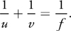
As the theoretical basis for our technique, we start from a virtual lens that focuses incoming light on an imaging plane. This lens is characterized by the focal length and the aperture. The focal length is the distance an imaging plane needs to be from the lens for parallel rays to map to a single point. The aperture is simply the diameter of the lens receiving light. The thin lens equation relates an object's distance from the lens u to the distance from the lens at which it is in focus v and the focal length of the lens f:

The geometry of a simple lens is shown in Figure 28-1. The aperture radius of the lens is d. The point u_o is in focus for the imaging plane, which is at v_o . A point at u_n or u_f would be in focus if the imaging plane were at v_f or v_n , respectively, but both map to a circle with diameter c when the imaging plane is at v_o . This circle is known as the circle of confusion. The depth of field for a camera is the range of values for which the CoC is sufficiently small.

Using similar triangles, we find that

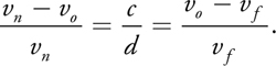
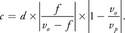
So, for any point in space p that is focused at v_p , we can specify its circle of confusion by

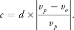
We can solve the thin lens approximation for v and substitute it into this equation to find the diameter of the circle of confusion for any point in space as a function of the camera's physical properties, as in Equation 1:

Equation 1

We are primarily concerned with the qualitative properties of this equation to convey a sense of limited depth of field. Specifically, we note the following:

• A "pinhole" camera model sets d to 0. In this case, c is always 0, so every point in space is always in focus. Any larger value of d will cause parts of the image to be out of focus. All real lenses, including the human eye, have d greater than 0.
• There is an upper bound on the diameter of the circle of confusion for points beyond the focal point.
• There is no upper bound on the circle of confusion closer than the focal point.
• The circle of confusion increases much more rapidly in the foreground than in the background.

28.4 Evolution of the Algorithm

Clearly, blurring objects near the camera is crucial to any convincing depth-of-field algorithm. Our algorithm evolved through various attempts at convincingly blurring nearby objects.

28.4.1 Initial Stochastic Approach

We started from the technique described in Scheuermann 2004. We calculated each pixel's circle of confusion independently and used that to scale a circular Poisson distribution of samples from the original image. Like Scheuermann, we also read the depth for each sample point, rejecting those too close to the camera.

This provides a very convincing blur for objects beyond the focal plane. Unfortunately, objects in front of the focal plane still have sharp silhouettes. Nearby objects do not appear out of focus—they just seem to have low-quality textures. This poor texture detracts from the player's experience, so it would be better to restrict ourselves to blurring distant objects than to use this technique for blurring the foreground.

This technique for blurring foreground objects is represented in the top right image of Figure 28-2. Note that the character's silhouette is unchanged from the reference image. This screenshot used 33 sample positions for 66 texture lookups per pixel, but it still suffers from ringing artifacts, particularly around the chin strap, the collar, and the eyes. Contrast this with the soft silhouette and smooth blur in the bottom right image.

28.4.2 The Scatter-as-Gather Approach

We considered the problem of blurring the background solved at this point, so we directed our efforts to bleeding blurry foreground objects past their silhouettes. Our first algorithm did a gather from neighboring pixels, essentially assuming that each neighbor had a CoC that was the same as the current one. Logically, we would prefer each pixel to smear itself over its neighbors based on its own circle of confusion.

This selectively sized smearing is a scattering operation, which doesn't map well to modern GPUs. We inverted this scattering operation into a gather operation by searching the neighborhood of each pixel for pixels that scattered onto it. We again sampled with a Poisson distribution, but because we were searching for the neighboring pixels that bleed onto the center pixel, we always had to use the maximum circle of confusion.

We found the CoC for each neighboring sample and calculated a weighted sum of only those samples that overlapped this pixel. Each sample's weight was inversely proportional to its area. We normalized the final color value by dividing by the sum of all used weights.

Unfortunately, this technique proved computationally and visually inadequate. We noticed that using less than about one-fourth of the pixels in the largest possible circle of confusion resulted in ugly ringing artifacts. This calculates to 24 sample points with 2 texture reads each for a maximum circle of confusion of only 5 pixels away (the diameter would be 11 pixels counting the center point). This cost could possibly be mitigated by using information about known neighbors to cull samples intelligently.

However, we abandoned this approach because it retained objectionable discontinuities between nearby unfocused pixels and more-distant focused pixels. To understand why this occurred, consider an edge between red source pixels with a large CoC and blue source pixels in focus. In the target image, the red pixels will have affected the blue pixels, but not vice versa. The unfocused red object will have a sharp silhouette against a purple background that fades to blue, instead of the continuous red-to-purple-to-blue transition we'd expect.

Two more problems with this method lead to the ugly behavior. First, the weight of each pixel should go smoothly to zero at the perimeter of the circle; without this, the output image will always have discontinuities where the blur radius changes. Second, the pixels cannot be combined using a simple normalized sum of their weights. To get the desired behavior, the contributing pixels need to be iterated from back to front, where this iteration's output color is a lerp from the previous iteration's output color to the current source pixel's color, based on the current source pixel's contribution weight. These two changes make this technique equivalent to rendering sorted depth sprites for each pixel with diameters equal to the pixel's CoC, essentially a post-process version of Kivánek et al. 2003. Unfortunately, they also make the pixel shader even more prohibitively expensive. Even with these fixes, the shader could not properly draw the scene behind any foreground objects that are blurred to transparency.

The bottom left image of Figure 28-2 was generated with this technique, using 64 sample points with a 12-pixel radius. The extra samples give this a better blur in the character's interior than the stochastic approach. However, 64 sample points are still too few for this blur radius, which leads to the ringing artifacts that can be seen on the antenna, neck, and helmet. Note that the silhouette still forms a harsh edge against the background; more samples wouldn't eliminate this.

28.4.3 The Blur Approach

At Infinity Ward we prioritize a quality user experience over an accurate simulation. That's why we abandoned physically based approaches when applying the circle of confusion for nearby objects in a continuous fashion. Instead, we decided to eliminate all discontinuities between focused objects and the unfocused foreground by using brute force, blurring them out of existence. The bottom right image in Figure 28-2 compares this technique to the previous approaches. The blur approach clearly has the best image quality, but it is also the fastest.

We apply a full-screen pass that calculates the radius of the circle of confusion for each foreground pixel into a render target. Pixels that are in focus or in the background use a CoC of zero. We then blur the CoC image to eliminate any edges. We use a Gaussian blur because it is computationally efficient and gives satisfactory results. We also downsample the CoC image to one-fourth the resolution along each axis as an optimization, so that the Gaussian blur affects only one-sixteenth of the total pixels in the frame.

This alone does not give the desired results for the silhouette of an unfocused object. If the foreground object is maximally blurred but the object behind it is not blurred at all, both objects will be approximately 50 percent blurred at their boundary. The foreground object should be 100 percent blurred along this edge. This does not look as bad as the previous discontinuities; however, it still looks odd when the blurriness of an edge on a foreground object varies based on the object behind it.

To fix this, we sized certain pixels—those located on either side of an edge between CoCs that had differing sizes—to always use the greater of the two diameters. However, a pixel has many neighbors, and we would rather avoid doing a search of all neighboring pixels. Instead, we only calculate each pixel's CoC and then use the blurred CoC image to estimate its neighboring pixel's CoC.

Consider an edge between two objects, each with uniform yet distinct circles of confusion having diameters D ₀ and D ₁. Clearly, in this case the blurred diameter D_B is given by

DB = (D 0 + D 1).

This equation also accurately gives the blurred diameter when the gradient of the diameter is the same on both sides of the edge, and for some other coincidental cases. We can get the current pixel's original diameter D ₀ and blurred diameter D_B in two texture lookups. From these, we estimate D ₁ by solving the previous equation:

D 1 2DB - D 0

Accordingly, we define our new diameter for the circle of confusion D by the equation

D = max(D 0, 2DB - D 0) = 2 max(D 0, DB ) - D 0.

Let D ₁ be the larger circle of confusion. This equation will transition smoothly from a diameter of D ₁ at the boundary between the two regions to D ₀ at the limits of the blur radius inside region 0. This is exactly what we want.

The maximum function is continuous when its inputs are continuous. The D ₀ input is not actually continuous, because it is the unblurred diameter for this pixel's circle of confusion. This function was chosen to be continuous along certain straight edges. Most straight-edge boundaries match these assumptions quite well within the blur radius. However, there are some objectionable discontinuities, particularly at 90-degree corners, so we apply one last small blur to fix this issue.

Figures 28-3 and 28-4 illustrate this process applied to a sample image. Each row is a particular sample image. The first column is the unprocessed image, and the second column is the image with the filter applied without the final blur. The third column is the final blurred result. Pure white in the input image represents the maximum circle of confusion; pixels that are black are in focus.

The first image is a simple black-and-white scene. Visually, these letters are floating in space very near the camera. The filter works well overall, but there are still some sharp edges at the corners of the letters, particularly in the uppercase "I". Blurring the image gets rid of the hard edge. It still leaves a gradient that is steeper than ideal, but it is good enough for our purposes.

The second row applies a small Gaussian blur to the sample image of the first row before applying the filter. This corresponds to looking at an object at a glancing angle. This results in a clear outline around the original image after it has been filtered. The final blur significantly dampens this artifact, but it doesn't completely fix it.

The final row applies a gradient to the original image. This corresponds to the typical case of an object that gradually recedes into the distance. The radius for the circle of confusion is overestimated in "valleys" and underestimated in "peaks," but it is continuous and there are none of the really objectionable artifacts from the second row. Again, the final blur dampens this artifact. Note that the gradient within the text is preserved.

28.5 The Complete Algorithm

Our completed algorithm consists of four stages:

1. Downsample the CoC for the foreground objects.
2. Blur the near CoC image.
3. Calculate the actual foreground CoC from the blurred and unblurred images.
4. Apply the foreground and background CoC image in one last full-screen pass that applies a variable-width blur.

28.5.1 Depth Information

Our algorithm is implemented using DirectX 9 hardware, which does not allow reading a depth buffer as a texture. We get around this limitation by binding a 32-bit floating-point color buffer during our depth pre-pass. Although we do not require full 32-bit precision, we picked that format because it is the least common denominator across all of our target hardware.

The pixel shader during depth pre-pass merely passes the world-space distance from the vertex shader through to the render target. In the pixel shader, we kill transparent pixels for 1-bit alpha textures by using the HLSL clip() intrinsic function.

In calling our technique a "pure post-process that can easily be plugged into an existing engine," we assume that the engine already generates this information. Our performance impact analysis also assumes that this information is already available. Our technique requires more than just applying post-processing modifications to a rendering engine if this assumption is invalid.

28.5.2 Variable-Width Blur

We need a fast variable-width blur to apply the circle of confusion to the scene. We could use a Poisson disk as in the original stochastic approach based on Scheuermann 2004. However, we generate the blur by approaching it differently. We consider that each pixel has a function that gives it its color based on the CoC diameter. We then approximate this function using a piecewise linear curve between three different blur radii and the original unblurred sample.

The two larger blur radii are calculated in the RGB channels at the same time the downsampled CoC is calculated in the alpha channel. The smallest blur radius is solved using five texture lookups, to average 17 pixels in a 5x5 grid, using the pattern in Figure 28-5.

Note that the center sample of this pattern reuses the texture lookup for the unblurred original pixel color.

This small blur is crucial for closely approximating the actual blur color. Without it, the image does not appear to blur continuously, but instead it appears to cross-fade with a blurred version of itself. We also found that a simple linear interpolation gave better results than a higher-polynomial spline because the splines tended to extrapolate colors for some pixels.

28.5.3 Circle of Confusion Radius

We are given the distance of each pixel to the camera in a depth texture. We see from Equation 1 that an accurate model of the radius for the circle of confusion can be calculated from this using only a reciprocal and a multiply-add instruction, with the engine providing suitable scale and bias constants.

However, we again take advantage of the freedom in computer simulation to forego physical plausibility in favor of artistic control. Artistically, we want some depth range to be in focus, with specific amounts of blur before and beyond it. It is unclear how to convert this into physical camera dimensions. The most intuitive way to edit this is by using a piecewise linear curve, as in Figure 28-6. The artists specify the near and far blur radii and the start and end distances for each of the three regions. We disable blurring for any region that has degenerate values, so artists can blur only the foreground or only the background if they wish.

In practice, we pick a world-near-end distance and a world-far-start distance that enclose everything that the player is likely to find of interest. We then set the world-near-start distance based on the world-near-end distance. Similarly, we set the world far-end distance based on the world-far-start distance.

28.5.4 First-Person Weapon Considerations

Infinity Ward develops first-person shooter games. The player's weapon (view model) is very important in these games because it is always in view and it is the primary way that the player interacts with the environment. DoF settings that looked good on the view model appeared to have no effect on the environment, while DoF settings that looked good on the nearby environment blurred the player's weapon excessively.

Our solution was to provide separate settings for the blur on the world and the player's view model. This makes no physical sense, but it provides a better experience for the player—perhaps because it properly conveys the effects of DoF whether the player is focusing on the important parts of the weapon or on the action in the environment. Each weapon configures its own near and far distances, with separate values used when the shooter aims with the weapon and when he or she holds it at the hip.

For this technique to work, we must know whether each pixel belongs to the view model or to the world. Our depth information is stored in a 32-bit floating-point render target. Using negative depths proved the most convenient way to get this bit of information. The normal lookup just requires a free absolute value modifier. This also leads to an efficient implementation for picking the near circle of confusion. We can calculate the near CoC for 4 pixels concurrently using a single mad_sat instruction. We calculate the near CoC for both the view model and the world in this way, and then we pick the appropriate CoC for all 4 pixels with a single min instruction.

28.5.5 The Complete Shader Listing

Most of the passes of our algorithm in Listing 28-1 are used to generate the near circle of confusion so that it is continuous and provides soft edges for foreground objects. We also want a large Gaussian blur radius, so we share GPU computation to concurrently calculate the blurred version of the scene and the near circle of confusion.

We specify the large blur radius in pixels at a normalized 480p resolution so that it is independent of actual screen resolution. However, the two small blurs are based on the actual screen resolution. We experimentally determined that the 17-tap small blur corresponds to a 1.4-pixel Gaussian blur at native resolution, and that the medium blur corresponds to a 3.6-pixel Gaussian blur at native resolution.

Example 28-1. A Shader That Downsamples the Scene and Initializes the Near CoC

    // These are set by the game engine.    // The render target size is one-quarter the scene rendering size.    sampler colorSampler; sampler depthSampler; const float2 dofEqWorld; const float2 dofEqWeapon; const float2 dofRowDelta;  // float2( 0, 0.25 / renderTargetHeight )    const float2 invRenderTargetSize; const float4x4 worldViewProj; struct PixelInput {   float4 position : POSITION;   float2 tcColor0 : TEXCOORD0;   float2 tcColor1 : TEXCOORD1;   float2 tcDepth0 : TEXCOORD2;   float2 tcDepth1 : TEXCOORD3;   float2 tcDepth2 : TEXCOORD4;   float2 tcDepth3 : TEXCOORD5; }; PixelInput DofDownVS( float4 pos : POSITION, float2 tc : TEXCOORD0 ) {   PixelInput pixel;   pixel.position = mul( pos, worldViewProj );   pixel.tcColor0 = tc + float2( -1.0, -1.0 ) * invRenderTargetSize;   pixel.tcColor1 = tc + float2( +1.0, -1.0 ) * invRenderTargetSize;   pixel.tcDepth0 = tc + float2( -1.5, -1.5 ) * invRenderTargetSize;   pixel.tcDepth1 = tc + float2( -0.5, -1.5 ) * invRenderTargetSize;   pixel.tcDepth2 = tc + float2( +0.5, -1.5 ) * invRenderTargetSize;   pixel.tcDepth3 = tc + float2( +1.5, -1.5 ) * invRenderTargetSize;   return pixel; } half4 DofDownPS( const PixelInput pixel ) : COLOR {   half3 color;   half maxCoc;   float4 depth;   half4 viewCoc;   half4 sceneCoc;   half4 curCoc;   half4 coc;   float2 rowOfs[4];   // "rowOfs" reduces how many moves PS2.0 uses to emulate swizzling.   rowOfs[0] = 0;   rowOfs[1] = dofRowDelta.xy;   rowOfs[2] = dofRowDelta.xy * 2;   rowOfs[3] = dofRowDelta.xy * 3;   // Use bilinear filtering to average 4 color samples for free.   color = 0;   color += tex2D( colorSampler, pixel.tcColor0.xy + rowOfs[0] ).rgb;   color += tex2D( colorSampler, pixel.tcColor1.xy + rowOfs[0] ).rgb;   color += tex2D( colorSampler, pixel.tcColor0.xy + rowOfs[2] ).rgb;   color += tex2D( colorSampler, pixel.tcColor1.xy + rowOfs[2] ).rgb;   color /= 4;   // Process 4 samples at a time to use vector hardware efficiently.    // The CoC will be 1 if the depth is negative, so use "min" to pick    // between "sceneCoc" and "viewCoc".   depth[0] = tex2D( depthSampler, pixel.tcDepth0.xy + rowOfs[0] ).r;   depth[1] = tex2D( depthSampler, pixel.tcDepth1.xy + rowOfs[0] ).r;   depth[2] = tex2D( depthSampler, pixel.tcDepth2.xy + rowOfs[0] ).r;   depth[3] = tex2D( depthSampler, pixel.tcDepth3.xy + rowOfs[0] ).r;   viewCoc = saturate( dofEqWeapon.x * -depth + dofEqWeapon.y );   sceneCoc = saturate( dofEqWorld.x * depth + dofEqWorld.y );   curCoc = min( viewCoc, sceneCoc );   coc = curCoc;   depth[0] = tex2D( depthSampler, pixel.tcDepth0.xy + rowOfs[1] ).r;   depth[1] = tex2D( depthSampler, pixel.tcDepth1.xy + rowOfs[1] ).r;   depth[2] = tex2D( depthSampler, pixel.tcDepth2.xy + rowOfs[1] ).r;   depth[3] = tex2D( depthSampler, pixel.tcDepth3.xy + rowOfs[1] ).r;   viewCoc = saturate( dofEqWeapon.x * -depth + dofEqWeapon.y );   sceneCoc = saturate( dofEqWorld.x * depth + dofEqWorld.y );   curCoc = min( viewCoc, sceneCoc );   coc = max( coc, curCoc );   depth[0] = tex2D( depthSampler, pixel.tcDepth0.xy + rowOfs[2] ).r;   depth[1] = tex2D( depthSampler, pixel.tcDepth1.xy + rowOfs[2] ).r;   depth[2] = tex2D( depthSampler, pixel.tcDepth2.xy + rowOfs[2] ).r;   depth[3] = tex2D( depthSampler, pixel.tcDepth3.xy + rowOfs[2] ).r;   viewCoc = saturate( dofEqWeapon.x * -depth + dofEqWeapon.y );   sceneCoc = saturate( dofEqWorld.x * depth + dofEqWorld.y );   curCoc = min( viewCoc, sceneCoc );   coc = max( coc, curCoc );   depth[0] = tex2D( depthSampler, pixel.tcDepth0.xy + rowOfs[3] ).r;   depth[1] = tex2D( depthSampler, pixel.tcDepth1.xy + rowOfs[3] ).r;   depth[2] = tex2D( depthSampler, pixel.tcDepth2.xy + rowOfs[3] ).r;   depth[3] = tex2D( depthSampler, pixel.tcDepth3.xy + rowOfs[3] ).r;   viewCoc = saturate( dofEqWeapon.x * -depth + dofEqWeapon.y );   sceneCoc = saturate( dofEqWorld.x * depth + dofEqWorld.y );   curCoc = min( viewCoc, sceneCoc );   coc = max( coc, curCoc );   maxCoc = max( max( coc[0], coc[1] ), max( coc[2], coc[3] ) );   return half4( color, maxCoc ); } 

We apply a Gaussian blur to the image generated by DofDownsample(). We do this with code that automatically divides the blur radius into an optimal sequence of horizontal and vertical filters that use bilinear filtering to read two samples at a time. Additionally, we apply a single unseparated 2D pass when it will use no more texture lookups than two separated 1D passes. In the 2D case, each texture lookup applies four samples. Listing 28-2 shows the code.

Example 28-2. A Pixel Shader That Calculates the Actual Near CoC

    // These are set by the game engine.    sampler shrunkSampler;  // Output of DofDownsample()    sampler blurredSampler; // Blurred version of the shrunk sampler    // This is the pixel shader function that calculates the actual    // value used for the near circle of confusion.    // "texCoords" are 0 at the bottom left pixel and 1 at the top right.    float4 DofNearCoc( const float2 texCoords ) {   float3 color;   float coc;   half4 blurred;   half4 shrunk;   shrunk = tex2D( shrunkSampler, texCoords );   blurred = tex2D( blurredSampler, texCoords );   color = shrunk.rgb;   coc = 2 * max( blurred.a, shrunk.a ) - shrunk.a;   return float4( color, coc ); } 

In Listing 28-3 we apply a small 3x3 blur to the result of DofNearCoc() to smooth out any discontinuities it introduced.

Example 28-3. This Shader Blurs the Near CoC and Downsampled Color Image Once

    // This vertex and pixel shader applies a 3 x 3 blur to the image in    // colorMapSampler, which is the same size as the render target.    // The sample weights are 1/16 in the corners, 2/16 on the edges,    // and 4/16 in the center.    sampler colorSampler;  // Output of DofNearCoc()    float2 invRenderTargetSize; struct PixelInput {   float4 position : POSITION;   float4 texCoords : TEXCOORD0; }; PixelInput SmallBlurVS( float4 position, float2 texCoords ) {   PixelInput pixel;   const float4 halfPixel = { -0.5, 0.5, -0.5, 0.5 };   pixel.position = Transform_ObjectToClip( position );   pixel.texCoords = texCoords.xxyy + halfPixel * invRenderTargetSize;   return pixel; } float4 SmallBlurPS( const PixelInput pixel ) {   float4 color;   color = 0;   color += tex2D( colorSampler, pixel.texCoords.xz );   color += tex2D( colorSampler, pixel.texCoords.yz );   color += tex2D( colorSampler, pixel.texCoords.xw );   color += tex2D( colorSampler, pixel.texCoords.yw );   return color / 4; } 

Our last shader, in Listing 28-4, applies the variable-width blur to the screen. We use a premultiplied alpha blend with the frame buffer to avoid actually looking up the color sample under the current pixel. In the shader, we treat all color samples that we actually read as having alpha equal to 1. Treating the unread center sample as having color equal to 0 and alpha equal to 0 inside the shader gives the correct results on the screen.

Example 28-4. This Pixel Shader Merges the Far CoC with the Near CoC and Applies It to the Screen

    sampler colorSampler;      // Original source image    sampler smallBlurSampler;  // Output of SmallBlurPS()    sampler largeBlurSampler;  // Blurred output of DofDownsample()    float2 invRenderTargetSize; float4 dofLerpScale; float4 dofLerpBias; float3 dofEqFar; float4 tex2Doffset( sampler s, float2 tc, float2 offset ) {   return tex2D( s, tc + offset * invRenderTargetSize ); } half3 GetSmallBlurSample( float2 texCoords ) {   half3 sum;   const half weight = 4.0 / 17;   sum = 0;  // Unblurred sample done by alpha blending   sum += weight * tex2Doffset( colorSampler, tc, +0.5, -1.5 ).rgb;   sum += weight * tex2Doffset( colorSampler, tc, -1.5, -0.5 ).rgb;   sum += weight * tex2Doffset( colorSampler, tc, -0.5, +1.5 ).rgb;   sum += weight * tex2Doffset( colorSampler, tc, +1.5, +0.5 ).rgb;   return sum; } half4 InterpolateDof( half3 small, half3 med, half3 large, half t ) {   half4 weights;   half3 color;   half  alpha;   // Efficiently calculate the cross-blend weights for each sample.    // Let the unblurred sample to small blur fade happen over distance    // d0, the small to medium blur over distance d1, and the medium to    // large blur over distance d2, where d0 + d1 + d2 = 1.    // dofLerpScale = float4( -1 / d0, -1 / d1, -1 / d2, 1 / d2 );    // dofLerpBias = float4( 1, (1 – d2) / d1, 1 / d2, (d2 – 1) / d2 );   weights = saturate( t * dofLerpScale + dofLerpBias );   weights.yz = min( weights.yz, 1 - weights.xy );   // Unblurred sample with weight "weights.x" done by alpha blending   color = weights.y * small + weights.z * med + weights.w * large;   alpha = dot( weights.yzw, half3( 16.0 / 17, 1.0, 1.0 ) );   return half4( color, alpha ); } half4 ApplyDepthOfField( const float2 texCoords ) {   half3 small;   half4 med;   half3 large;   half depth;   half nearCoc;   half farCoc;   half coc;   small = GetSmallBlurSample( texCoords );   med = tex2D( smallBlurSampler, texCoords );   large = tex2D( largeBlurSampler, texCoords ).rgb;   nearCoc = med.a;   depth = tex2D( depthSampler, texCoords ).r;   if ( depth > 1.0e6 )   {     coc = nearCoc; // We don't want to blur the sky.   }   else   {     // dofEqFar.x and dofEqFar.y specify the linear ramp to convert    // to depth for the distant out-of-focus region.    // dofEqFar.z is the ratio of the far to the near blur radius.     farCoc = saturate( dofEqFar.x * depth + dofEqFar.y );     coc = max( nearCoc, farCoc * dofEqFar.z );   }   return InterpolateDof( small, med.rgb, large, coc ); } 

28.6 Conclusion

Not much arithmetic is going on in these shaders, so their cost is dominated by the texture lookups.

• Generating the quarter-resolution image uses four color lookups and 16 depth lookups for each target pixel in the quarter-resolution image, equaling 1.25 lookups per pixel in the original image.
• The small radius blur adds another four lookups per pixel.
• Applying the variable-width blur requires reading a depth and two precalculated blur levels, which adds up to three more lookups per pixel.
• Getting the adjusted circle of confusion requires two texture lookups per pixel in the quarter-resolution image, or 0.125 samples per pixel of the original image.
• The small blur applied to the near CoC image uses another four texture lookups, for another 0.25 samples per pixel in the original.

This equals 8.625 samples per pixel, not counting the variable number of samples needed to apply the large Gaussian blur. Implemented as a separable filter, the blur will typically use no more than two passes with eight texture lookups each, which gives 17 taps with bilinear filtering. This averages out to one sample per pixel in the original image. The expected number of texture lookups per pixel is about 9.6.

Frame-buffer bandwidth is another consideration. This technique writes to the quarter-resolution image once for the original downsample, and then another two times (typically) for the large Gaussian blur. There are two more passes over the quarter-resolution image—to apply Equation 1 and to blur its results slightly. Finally, each pixel in the original image is written once to get the final output. This works out to 1.3125 writes for every pixel in the original image.

Similarly, there are six render target switches in this technique, again assuming only two passes for the large Gaussian blur.

The measured performance cost was 1 to 1.5 milliseconds at 1024x768 on our tests with a Radeon X1900 and GeForce 7900. The performance hit on next-generation consoles is similar. This is actually faster than the original implementation based on Scheuermann 2004, presumably because it uses fewer than half as many texture reads.

28.7 Limitations and Future Work

When you use our approach, focused objects will bleed onto unfocused background objects. This is the least objectionable artifact with this technique and with post-process DoF techniques in general. These artifacts could be reduced by taking additional depth samples for the 17-tap blur. This should be adequate because, as we have seen, the background needs to use a smaller blur radius than the foreground.

The second artifact is inherent to the technique: You cannot increase the blur radius for near objects so much that it becomes obvious that the technique is actually a blur of the screen instead of a blur of the unfocused objects. Figure 28-7 is a worst-case example of this problem, whereas Figure 28-8 shows a more typical situation. The center image in Figure 28-8 shows a typical blur radius. The right image has twice that blur radius; even the relatively large rock in the background has been smeared out of existence. This becomes particularly objectionable as the camera moves, showing up as a haze around the foreground object.

The radius at which this happens depends on the size of the object that is out of focus and the amount of detail in the geometry that should be in focus. Smaller objects that are out of focus, and focused objects that have higher frequencies, require a smaller maximum blur radius. This could be overcome by rendering the foreground objects into a separate buffer so that the color information that gets blurred is only for the foreground objects. This would require carefully handling missing pixels. It also makes the technique more intrusive into the rendering pipeline.

Finally, we don't explicitly handle transparency. Transparent surfaces use the CoC of the first opaque object behind them. To fix this, transparent objects could be drawn after depth of field has been applied to all opaque geometry. They could be given an impression of DoF by biasing the texture lookups toward lower mipmap levels. Particle effects may also benefit from slightly increasing the size of the particle as it goes out of focus. Transparent objects that share edges with opaque objects, such as windows, may still have some objectionable artifacts at the boundary. Again, this makes the technique intrusive. We found that completely ignoring transparency works well enough in most situations.

28.8 References

Demers, Joe. 2004. "Depth of Field: A Survey of Techniques." In GPU Gems, edited by Randima Fernando, pp. 375–390. Addison-Wesley.

Kass, Michael, Aaron Lefohn, and John Owens. 2006. "Interactive Depth of Field Using Simulated Diffusion on a GPU." Technical report. Pixar Animation Studios. Available online at http://graphics.pixar.com/DepthOfField/paper.pdf.

Kosloff, Todd Jerome, and Brian A. Barsky. 2007. "An Algorithm for Rendering Generalized Depth of Field Effects Based On Simulated Heat Diffusion." Technical Report No. UCB/EECS-2007-19. Available online at http://www.eecs.berkeley.edu/Pubs/TechRpts/2007/EECS-2007-19.pdf.

Kivánek, Jaroslav, Jií ára, and Kadi Bouatouch. 2003. "Fast Depth of Field Rendering with Surface Splatting." Presentation at Computer Graphics International 2003. Available online at http://www.cgg.cvut.cz/~xkrivanj/papers/cgi2003/9-3_krivanek_j.pdf.

Mulder, Jurriaan, and Robert van Liere. 2000. "Fast Perception-Based Depth of Field Rendering." Available online at http://www.cwi.nl/~robertl/papers/2000/vrst/paper.pdf.

Potmesil, Michael, and Indranil Chakravarty. 1981. "A Lens and Aperture Camera Model for Synthetic Image Generation." In Proceedings of the 8th Annual Conference on Computer Graphics and Interactive Techniques, pp. 297–305.

Scheuermann, Thorsten. 2004. "Advanced Depth of Field." Presentation at Game Developers Conference 2004. Available online at http://ati.amd.com/developer/gdc/Scheuermann_DepthOfField.pdf.

• Contributors
• Foreword
• Part I: Geometry
• Chapter 1. Generating Complex Procedural Terrains Using the GPU
• Chapter 2. Animated Crowd Rendering
• Chapter 3. DirectX 10 Blend Shapes: Breaking the Limits
• Chapter 4. Next-Generation SpeedTree Rendering
• Chapter 5. Generic Adaptive Mesh Refinement
• Chapter 6. GPU-Generated Procedural Wind Animations for Trees
• Chapter 7. Point-Based Visualization of Metaballs on a GPU
• Part II: Light and Shadows
• Chapter 8. Summed-Area Variance Shadow Maps
• Chapter 9. Interactive Cinematic Relighting with Global Illumination
• Chapter 10. Parallel-Split Shadow Maps on Programmable GPUs
• Chapter 11. Efficient and Robust Shadow Volumes Using Hierarchical Occlusion Culling and Geometry Shaders
• Chapter 12. High-Quality Ambient Occlusion
• Chapter 13. Volumetric Light Scattering as a Post-Process
• Part III: Rendering
• Chapter 14. Advanced Techniques for Realistic Real-Time Skin Rendering
• Chapter 15. Playable Universal Capture
• Chapter 16. Vegetation Procedural Animation and Shading in Crysis
• Chapter 17. Robust Multiple Specular Reflections and Refractions
• Chapter 18. Relaxed Cone Stepping for Relief Mapping
• Chapter 19. Deferred Shading in Tabula Rasa
• Chapter 20. GPU-Based Importance Sampling
• Part IV: Image Effects
• Chapter 21. True Impostors
• Chapter 22. Baking Normal Maps on the GPU
• Chapter 23. High-Speed, Off-Screen Particles
• Chapter 24. The Importance of Being Linear
• Chapter 25. Rendering Vector Art on the GPU
• Chapter 26. Object Detection by Color: Using the GPU for Real-Time Video Image Processing
• Chapter 27. Motion Blur as a Post-Processing Effect
• Chapter 28. Practical Post-Process Depth of Field
• Part V: Physics Simulation
• Chapter 29. Real-Time Rigid Body Simulation on GPUs
• Chapter 30. Real-Time Simulation and Rendering of 3D Fluids
• Chapter 31. Fast N-Body Simulation with CUDA
• Chapter 32. Broad-Phase Collision Detection with CUDA
• Chapter 33. LCP Algorithms for Collision Detection Using CUDA
• Chapter 34. Signed Distance Fields Using Single-Pass GPU Scan Conversion of Tetrahedra
• Chapter 35. Fast Virus Signature Matching on the GPU
• Part VI: GPU Computing
• Chapter 36. AES Encryption and Decryption on the GPU
• Chapter 37. Efficient Random Number Generation and Application Using CUDA
• Chapter 38. Imaging Earth's Subsurface Using CUDA
• Chapter 39. Parallel Prefix Sum (Scan) with CUDA
• Chapter 40. Incremental Computation of the Gaussian
• Chapter 41. Using the Geometry Shader for Compact and Variable-Length GPU Feedback
• Preface