GPU Gems 3

GPU Gems 3 is now available for free online!

The CD content, including demos and content, is available on the web and for download.

You can also subscribe to our Developer News Feed to get notifications of new material on the site.

Chapter 37. Efficient Random Number Generation and Application Using CUDA

Lee Howes
Imperial College London

David Thomas
Imperial College London

Monte Carlo methods provide approximate numerical solutions to problems that would be difficult or impossible to solve exactly. The defining characteristic of Monte Carlo simulations is the use of multiple independent trials, each driven by some stochastic (random) process. The results of the independent trials are then combined to extract the average answer, relying on the Law of Large Numbers, which states that as more trials are combined, the average answer will converge on the true answer. The independent trials are inherently parallelizable, and they typically consist of dense numeric operations, so GPUs provide an almost ideal platform for Monte Carlo simulations.

However, a key component within Monte Carlo simulations is the random number generators (RNGs) that provide the independent stochastic input to each trial. These generators must meet the conflicting goals of being extremely fast while also providing random number streams that are indistinguishable from a true random number source. There is an extensive body of literature devoted to random number generation in CPUs, but the most efficient of these make fundamental assumptions about processor architecture and performance: they are often not appropriate for use in GPUs. Previous work such as Sussman et. al. 2006 has investigated random number generation in older generations of GPUs, but the latest generation of completely programmable GPUs has different characteristics, requiring a new approach.

In this chapter, we discuss methods for generating random numbers using CUDA, with particular regard to generation of Gaussian random numbers, a key component of many financial simulations. We describe two methods for generating Gaussian random numbers, one of which works by transforming uniformly distributed numbers using the Box-Muller method, and another that generates Gaussian distributed random numbers directly using the Wallace method. We then demonstrate how these random number generators can be used in real simulations, using two examples of valuing exotic options using CUDA. Overall, we find that a single GeForce 8 GPU generates Gaussian random numbers 26 times faster than a Quad Opteron 2.2 GHz CPU, and we find corresponding speedups of 59x and 23x in the two financial examples.

37.1 Monte Carlo Simulations

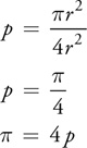
Monte Carlo approaches were introduced by Ulam and von Neumann in the 1940s with the aim of simulating nuclear reactions (Metropolis 1987). A simple example of a Monte Carlo solution to a problem is for calculating . Take a square and inscribe within it a circle that touches each edge of the square. We know that if the radius of the circle is r, then the area of the circle is r ², and the area of the square is 4r ². If we can calculate the ratio, p, of the circle area to the square area, then we can calculate :

We can calculate the ratio p using Monte Carlo methods by generatingn independent random points that are uniformly distributed within the square. Some fraction k of the points will lie within the circle, thus we have p k/n, leading to p 4k/n. Figure 37-1 shows random points placed within a circle, with n = 20, 200, and 2,000, shown as blue circles, red crosses, and green points, respectively, providing estimates of as 3.4, 3.18, and 3.158. As the number of points increases, the accuracy improves, giving estimates of 3.1492 for n = 2 x 10⁴ and 3.1435 for n = 2 x 10⁵.

Figure 37-1 Random Points Within a Square to Calculate Pi

Clearly this is an inefficient way to calculate : the rate of increase in accuracy is low (accuracy is usually proportional to the square root of the number of trials) and is much less efficient than standard iterative methods. However, it does demonstrate three reasons why Monte Carlo methods are so popular:

It is very easy to understand how the method works, which is often not the case with the algorithm for the corresponding exact solution (assuming one exists).
It is very easy to implement, with the main hurdle being the generation of random numbers.
Monte Carlo methods are inherently parallelizable.

This last point is a major advantage, allowing Monte Carlo solutions to easily scale to multiple nodes in a networked cluster, or to multiple processors within a CPU or GPU.

A more realistic example of Monte Carlo methods is in finance. Here the approach is to capture a subset of market variables—for example, the price S ₀ of an equity at time 0—then choose an artificial stochastic model that appears to model previous equity paths reasonably well. The most commonly used model is geometric Brownian motion, where the final price of the stock at time t is modeled as S_t = S ₀ e ^{µ+ N} , where N is a random sample from the Gaussian distribution (Wilmott 2006).

A programmatic estimator of the average stock price would then be as shown in Listing 37-1. The goal of the random runs is to produce an approximation to the behavior of the historical market and use the results to judge the probability of making a profit. This is similar to the computation example, where the system tends toward the probability of a point being within the circle, and that probability is directly related to the ratio of areas. This method allows us to find solutions for a wide class of financial models for which there are no analytical solutions.

Example 37-1. Estimating the Average Stock Price

    float sum=0; for(unsigned i=0;i<N;i++){   sum += S0 * exp(mu+sigma*RandN()); } return sum/N;

The Monte Carlo approach is trivially parallelizable across multiple processors, and it is often called embarrassingly parallel. There are five major steps:

Assign each processing element a random sequence. Each processing element must use a different random number sequence, which should be uncorrelated with the sequences used by all other processors.
Propagate the simulation parameters (for example, S ₀) to all processing elements, and tell them how many simulation runs to execute.
Generate random number streams for use by each processing element.
Execute the simulation kernel on the processing elements in parallel.
Gather the simulation outputs from each processing element and combine them to produce the approximate results.

In many traditional architectures, the difficult part is step 4, writing an efficient implementation of the simulation kernel, because a faster kernel allows more simulated trials to be executed within a given time and so will provide a more accurate answer. However, in a GPU, the mathematically heavy simulation kernel is often relatively easy to implement. The real challenge is to manage the assignment of different random number streams to processors, and to generate those random number streams efficiently. Figure 37-2 shows the division of processing among processors at a high level.

Figure 37-2 Dividing the Simulation Space Among Multiple Executions of the Simulation Kernel

37.2 Random Number Generators

37.2.1 Introduction

Random number generators can be classified into three groups, according to the source of their "randomness":

True random number generators (TRNGs). This type uses a physical source of randomness to provide truly unpredictable numbers. TRNGs are mainly used for cryptography, because they are too slow for simulation purposes.
Quasirandom number generators (QRNGs). These generators attempt to evenly fill an n-dimensional space with points, without clustering or grouping of points. Although QRNGs are used in Monte Carlo simulations, we do not consider them in this chapter.
Pseudorandom number generators (PRNGs). The most common type of random number generator, PRNGs are designed to look as random as a TRNG, but can be implemented in deterministic software because the state and transition function can be predicted completely. In this chapter, we consider only this type of generator.

An orthogonal classification of random number generators is organized according to the distribution of the numbers that are produced. Commonly encountered library functions, such as C's rand(), sample from the uniform distribution, meaning that within some range of numbers, each value is equally likely to occur.

However, many Monte Carlo simulations actually need different distributions; common examples are the normal, log-normal, and exponential distributions. The main method used for producing samples from nonuniform distributions is first to generate uniform random numbers, and then to apply a transform to convert the uniform numbers into samples from the desired nonuniform distribution.

To give an example, a standard exponential variate E has the cumulative distribution function (CDF) F_E (x) = P[x < E ] = 1 - e ^-x . The CDF maps a sample x from the exponential distribution back to the probability of a value less than x occurring, where the probability is a value between 0 and 1. Thus if E is exponentially distributed, then P[x < E ] will be uniformly distributed. This leads to the inversion method: if we know that F_E (x) converts from the exponential distribution to the uniform distribution, then logically will convert from the uniform distribution to the exponential distribution. Thus if a random variate U is uniformly distributed, then will be exponentially distributed.

Although inverting the CDF is a conceptually simple method, it is often too computationally expensive to use. In the preceding exponential example, a call to log() is required for every random number. This may be acceptable, but in many cases the inverse may be much more complicated, or in some cases there may not even be a closed-form solution. This is the case for the Gaussian distribution, one of the most important distributions, so significant effort has been devoted to investigating alternative methods for transforming the uniform distribution. Rather than use the direct inverse CDF transform, these methods use mathematical identities and statistical tricks to convert from the uniform distribution, for example by using pairs of uniform random numbers.

We then see two main general requirements that we wish PRNGs to satisfy:

A long period. Every deterministic generator must eventually loop, but the goal is to make the loop period as long as possible. There is a strong argument that if n random samples are used across all nodes in a simulation, then the period of the generator should be at least n ².
Good statistical quality. The output from the generator should be practically indistinguishable from a TRNG of the required distribution, and it should not exhibit any correlations or patterns. Poor generator quality can ruin the results of Monte Carlo applications, and it is critical that generators are able to pass the set of theoretical and empirical tests for quality that are available. Numerous statistical tests are available to verify this requirement (Knuth 1969, Marsaglia 1995, L'Ecuyer 2006).

In this chapter, we consider two methods for generating Gaussian random numbers that are particularly well suited to the new class of GPUs. The first uses the traditional technique of generating uniform random numbers, then applying a transform to produce the Gaussian distribution. The second uses a newer technique to generate random numbers directly, without needing a uniform random source. We then look at the use of these generators within two Monte Carlo simulations for exotic option valuation.

37.2.2 Uniform-to-Gaussian Conversion Generator

The traditional method for producing Gaussian random numbers requires two components: a uniform PRNG and a transform to the Gaussian distribution. There are many choices for both components, so here we briefly discuss the requirements for each, and provide a brief analysis of the main choices. We will then select two components based on the unique requirements of GPU architectures.

Besides meeting the general requirements of uniform PRNGs discussed in Section 37.2.1, the parallel nature of GPUs imposes two additional requirements:

The ability to generate different substreams on parallel nodes. Each node must be given a different portion of the random stream with no overlap.
No correlations between substreams on different nodes. The substreams must appear to be completely independent streams of random numbers.

Available Uniform PRNGs

Linear Congruential Generator

The classic generator is the linear congruential generator (LCG) (Knuth 1969), which uses a transition function of the form x_n ₊ ₁ = (ax_n +c) mod m. The maximum period of the generator is m (assuming the triple (a, c, m) has certain properties), but this means that in a 32-bit integer, the period can be at most 2³², which is far too low. LCGs also have known statistical flaws, making them unsuitable for modern simulations.

Multiple Recursive Generator

A derivative of the LCG is the multiple recursive generator (MRG), which additively combines two or more generators. If n generators with periods m ₁, m ₂, . . ., m_n are combined, then the resulting period is LCM(m ₁, m ₂, . . ., m_n ), thus the period can be at most m ₁ x, m ₂ x, . . ., m_nx. These generators provide both good statistical quality and long periods, but the relatively prime moduli require complex algorithms using 32-bit multiplications and divisions, so they are not suitable for current GPUs (NVIDIA 2007, Section 6.1.1.1).

Lagged Fibonacci Generator

A generator that is commonly used in distributed Monte Carlo simulations is the lagged Fibonacci generator (Knuth 1969). This generator is similar to an LCG but introduces a delayed feedback, using the transition function x_n ₊₁ = (x_n x_n _- _k ) modm, where is typically addition or multiplication. However, to achieve good quality, the constant k must be large. Consequentially k words of memory must be used to hold the state. Typically k must be greater than 1000, and each thread will require its own state, so this must be stored in global memory. We thus reject the lagged Fibonacci method but note that it may be useful in some GPU-based applications, because of the simplicity and small number of registers required.

Mersenne Twister

One of the most widely respected methods for random number generation in software is the Mersenne twister (Matsumoto and Nishimura 1998), which has a period of 2^19,937 and extremely good statistical quality. However, it presents problems similar to those of the lagged Fibonacci, because it has a large state that must be updated serially. Thus each thread must have an individual state in global RAM and make multiple accesses per generator. In combination with the relatively large amount of computation per generated number, this requirement makes the generator too slow, except in cases where the ultimate in quality is needed.

Combined Tausworthe Generator

Internally, the Mersenne twister utilizes a binary matrix to transform one vector of bits into a new vector of bits, using an extremely large sparse matrix and large vectors. However, there are a number of related generators that use much smaller vectors, of the order of two to four words, and a correspondingly denser matrix. An example of this kind of generator is the combined Tausworthe generator, which uses exclusive-or to combine the results of two or more independent binary matrix derived streams, providing a stream of longer period and much better quality. Each independent stream is generated using TausStep, shown in Listing 37-2, in six bitwise instructions. For example, the four-component LFSR113 generator from L'Ecuyer 1999 requires 6 x 4 + 3 = 27 instructions, producing a stream with a period of approximately 2¹¹³.

Example 37-2. A Single Step of the Combined Tausworthe Generator

    // S1, S2, S3, and M are all constants, and z is part of the    // private per-thread generator state.    unsigned TausStep(unsigned &z, int S1, int S2, int S3, unsigned M) {   unsigned b=(((z << S1) ^ z) >> S2);   return z = (((z & M) << S3) ^ b); }

However, our statistical tests show that even the four-component LFSR113 produces significant correlations across 5-tuples and 6-tuples, even for relatively small sample sizes.

A Hybrid Generator

The approach we propose is to combine the simple combined Tausworthe with another kind of generator; if the periods of all the components are co-prime, then the resulting generator period will be the product of all the component periods, and the statistical defects of one generator should hide those of the other.

We have already mentioned LCG-based generators but dismissed them because of the prime moduli needed to create MRGs. However, if we use a single generator with a modulus of 2³², we gain two important properties: (1) The modulus is applied for free in LCGStep, shown in Listing 37-3, due to the truncation in 32-bit arithmetic. (2) The resulting period of 2³² is relatively prime to all the component periods of a combined Tausworthe, thus the two can be combined to create a much longer period generator.

Example 37-3. A Simple Linear Congruential Generator

    // A and C are constants    unsigned LCGStep(unsigned &z, unsigned A, unsigned C) {   return z=(A*z+C); }

The specific combination we chose is the three-component combined Tausworthe "taus88" from L'Ecuyer 1996 and the 32-bit "Quick and Dirty" LCG from Press et al. 1992, as shown in Listing 37-4. Both provide relatively good statistical quality within each family of generators, and in combination they remove all the statistical defects we observed in each separate generator. The generator state comprises four 32-bit values, and it provides an overall period of around 2¹²¹. The only restrictions on the initial state are that the three Tausworthe state components should be greater than 128; other than that, the four state components can be initialized to any random values. Each thread should receive a different set of four state values, which should be uncorrelated and for convenience can be supplied using a CPU-side random number generator. For cases in which a significant fraction of the entire random stream will be used (for example, more than 2⁶⁴), it is possible to use stream skipping to advance each of the four state components, ensuring independent random streams; however, that case is out of the scope of this chapter.

Example 37-4. Combining the LCG and Tausworthe into an Improved Generator

    unsigned z1, z2, z3, z4; float HybridTaus() {   // Combined period is lcm(p1,p2,p3,p4)~ 2^121    return 2.3283064365387e-10 * (              // Periods     TausStep(z1, 13, 19, 12, 4294967294UL) ^  // p1=2^31-1     TausStep(z2, 2, 25, 4, 4294967288UL) ^    // p2=2^30-1     TausStep(z3, 3, 11, 17, 4294967280UL) ^   // p3=2^28-1     LCGStep(z4, 1664525, 1013904223UL)        // p4=2^32    ); }

KISS

Another well-respected hybrid generator is the KISS family (L'Ecuyer 2006) from Marsaglia. These combine three separate types of generator: an LCG, a shift-based generator similar to the Tausworthe, and a pair of multiply-with-carry generators. Although this generator also gives good statistical quality, it requires numerous 32-bit multiplications, which harm performance (NVIDIA 2007, Section 6.1.1.1) on current-generation hardware, offering only 80 percent of the Tausworthe's performance.

37.2.3 Types of Gaussian Transforms

We now turn to the transformation from the uniform to Gaussian distribution. Again, there are many techniques to choose from, because the Gaussian distribution is so important.

The Ziggurat Method

The fastest method in software is the ziggurat method (Marsaglia 2000). This procedure uses a complicated method to split the Gaussian probability density function into axisaligned rectangles, and it is designed to minimize the average cost of generating a sample. However, this means that for 2 percent of generated numbers, a more complicated route using further uniform samples and function calls must be made. In software this is acceptable, but in a GPU, the performance of the slow route will apply to all threads in a warp, even if only one thread uses the route. If the warp size is 32 and the probability of taking the slow route is 2 percent, then the probability of any warp taking the slow route is (1 - 0.02)³², which is 47 percent! So, because of thread batching, the assumptions designed into the ziggurat are violated, and the performance advantage is destroyed.

The Polar Method

Many other methods also rely on looping behavior similar to that of the Ziggurat and so are also not usable in hardware. The polar method (Press et. al. 1992) is simple and relatively efficient, but the probability of looping per thread is 14 percent. This leads to an expected 1.6 iterations per generated sample turning into an expected 3.1 iterations when warp effects are taken into account.

The Box-Muller Transform

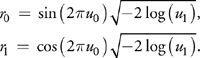
Because GPUs are so sensitive to looping and branching, it turns out that the best choice for the Gaussian transform is actually the venerable Box-Muller transform, code for which can be seen in Listing 37-5. This takes two uniform samples u0 and u1 and transforms them into two Gaussian distributed samples n0 and n1, using the relations:

Example 37-5. The Box-Muller Transform

    float2 BoxMuller() {   float u0=HybridTaus (), u1=HybridTaus ();   float r=sqrt(-2 log(u0));   float theta=2*PI*u1;   return make_float2(r*sin(theta),r*cos(theta)); }

The Box-Muller approach has been largely discarded in software, in particular because it requires the evaluation of sine and cosine for every sample that is produced. However, it offers a number of important advantages for a GPU implementation with batched threads, the most obvious of which is that it has no branching or looping: there is only a single code path. It also does not require any table lookups, or the large numbers of constants found in some methods. It still has a fairly high computational load, but fortunately this is what GPUs are good at: straight-line code, loaded with math. In addition, our results suggest that the high-speed sine and cosine functions present on the GPU offer satisfactory results, largely negating the performance downsides of the Box-Muller approach.

37.2.4 The Wallace Gaussian Generator

The Wallace Gaussian generator(Wallace 1996, Brent 2003) is a novel method that is able to generate Gaussian samples directly, without using a uniform generator first. The central idea is to take a pool of k random numbers that are already Gaussian distributed and then apply a transform to the pool, such that another pool is produced that is also Gaussian. After each transform the pool can be output to supply random numbers. The key requirement is to make the output of the transform as uncorrelated with the input as possible, while still preserving the distribution properties.

Ideally each new pool would be produced by applying a different orthogonal kxk matrix to the previous pool. An orthogonal matrix is one that preserves the sum of squares in the pool, or put another way: if the input pool is taken as a k-dimensional vector, then an orthogonal matrix would preserve the Euclidean length of that vector. Common examples of orthogonal matrices include the identity matrix and size-preserving affine transforms such as reflection and rotation.

However, there is a computational problem, because generating a random kxk orthogonal matrix is very expensive—orders of magnitude more expensive than just generating k Gaussian-distributed numbers using traditional techniques. Instead, the approach used is to construct an orthogonal transform using lots of much smaller orthogonal transforms, for example by using 2x2 orthogonal matrices, such as 2D rotations. Applying k/2 2D rotations will preserve the length of the overall k vector, but it is much cheaper to implement. The drawback is that the degree of mixing between passes is much lower: using a full kxk matrix, each value in the new pool can be influenced by every value in the old pool, but if 2x2 matrices are used, then each value in the new pool depends on at most two values in the old pool.

Two techniques can mitigate this lack of mixing. The first applies a random permutation to the pool before applying the blocked transform, so that after a sufficient number of passes, each element of the new pool will be dependent on all elements of a previous pool. The second simply transforms the pool multiple times before using the pool to output numbers. Both methods have their drawbacks, because a full random permutation is expensive to set up, and performing multiple passes obviously takes more time. In practice, a combination of both is often used, performing a small number of passes and using a somewhat random permutation of the pool in each pass.

Figure 37-3 A Single Step of the Wallace Transform

Permuting the Pool

Mapping the Wallace algorithm into a GPU presents a number of challenges. The most important requirement is that the random permutation must be sufficiently random. In tests we found that the quality of this permutation was a key factor in producing goodquality random numbers: using simple nonrandom permutations produced random numbers that failed statistical tests. In light of these tests, we determined that producing a random permutation was much more important than reducing bank conflicts, so we can ignore conflicts when designing the algorithm.

The only critical requirement for the permutation is that it must be exactly that, a permutation. No pool value can be read twice during a pass (and so logically, no pool value can be ignored). During the reading stage, each thread must read d samples from a pool of k samples. We can thus define the problem as creating a random mapping from 1..k 1..dx 1..k/d. Earlier we mentioned the LCG, which provides a method for specifying a maximum period generator in the range [0,m). If we choose m =k/d, we can use this as the basis of a high-quality random permutation.

We already have a unique per-thread value, the thread id, which is a value in [0,m). Now, if we take the thread id and feed it into a mod-m LCG, each thread will still have a unique identifier, but the ordering will have changed pseudorandomly. Note that this LCG provides low statistical quality; however, we found that in this context, low quality is not a problem. Applying the LCG again would result in a new mapping, but each thread would still have a unique identifier in the range [0, m). The combination of the address permutation and the blockwise orthogonal transformation forms the basis of the transformation process. When we combine an individual Wallace transform step with a loop to perform repeated internal transformations as part of an overall visible transformation, we obtain the code in Listing 37-6, where TransformBlock performs the matrix operation on the data, in this case using a Walsh-Hadamard matrix (Wallace 1996).

Example 37-6. Transforming the Wallace Pool Using a Defined Number of Passes and a Walsh-Hadamard Matrix on Each Set of Values

This uses a defined number of passes and a Walsh-Hadamard matrix on each set of values. The size of the block to execute a matrix on can be varied but for optimality should use registers, and hence we have manually unrolled the computation here.

    void Transform() {   // K, and M are binary powers.    const unsigned K=...;  // Size of pool    const unsigned M=K/D;  // Number of threads, and LCG modulus    float block_0, block_1 , block_2 , block_3;   for( int pass = 0; pass < POOL_PASSES; pass++ ) {     // Read the pool in using a pseudorandom permutation.    unsigned s=tid;     // M is a binary power, don't need %.    // s is being recomputed as an LCG.     s = (s*A+B) & (M-1); block_0=pool[(s<<3)+0];     s = (s*A+B) & (M-1); block_1=pool[(s<<3)+1];     s = (s*A+B) & (M-1); block_2=pool[(s<<3)+2];     s = (s*A+B) & (M-1); block_3=pool[(s<<3)+3];     // All pool values must be read before any are written.    __syncthreads();     // Perform in-place 4x4 orthogonal transform on block.     TransformBlock(block);     // Output the blocks in linear order.     s=tid;     pool[s]=block_0; s+=NT;     pool[s]=block_1; s+=NT;     pool[s]=block_2; s+=NT;     pool[s]=block_3; s+=NT;   } } __device__ void TransformBlock(float *b) {   float t=(b[0]+b[1]+b[2]+b[3])/2;   b[0]=b[0]-t;   b[1]=b[1]-t;   b[2]=t-b[2];   b[3]=t-b[3]; }

Initializing the Pool

Initialization of the random number pool is necessarily a separate process from the Wallace generator itself and hence requires a separate random number generator. This initialization can be performed on the CPU: for example, by using the ziggurat method in concert with a Mersenne twister. Although this generator will not be as fast as the GPU-based Wallace generator, it needs to provide only the seed values for the Wallace pools; once the threads start executing, they require no further seed values. In fact, the software can take advantage of this by generating the next set of seed values while the GPU threads work from the previous set of seed values.

The Wallace approach to random number generation conveys two main advantages over other approaches:

Direct generation of normally distributed values
A state pool that can be operated on fully in parallel, allowing high utilization of processor-local shared memory resources

37.2.5 Integrating the Wallace Gaussian Generator into a Simulation

Listing 37-7 demonstrates how the Wallace transform can be combined with code to perform repeated passes and to output multiple random numbers per execution into global memory. It is, of course, no problem to replace the global memory output with the use of the values within a simulation. Because we have generated multiple random numbers in each thread (the entire matrix size at a minimum), we can use these repeatedly within the transform, taking the appropriate pool value from shared memory as needed.

Example 37-7. Using the Wallace Generator to Output into Memory

Note that an array of chi² correction values is required to maintain statistical properties of the output data. A small performance improvement can be obtained by moving this data into constant memory (around 5 percent in this case), thanks to caching. Constant memory is limited in size and hence care must be taken with this adjustment.

    __device__ void generateRandomNumbers_wallace(   unsigned seed,  // Initialization seed    float *chi2Corrections,  // Set of correction values    float *globalPool,  // Input random number pool    float *output  // Output random numbers ){   unsigned tid=threadIdx.x;   // Load global pool into shared memory.    unsigned offset = __mul24(POOL_SIZE, blockIdx.x);   for( int i = 0; i < 4; i++ )     pool[tid+THREADS*i] = globalPool[offset+TOTAL_THREADS*i+tid];   __syncthreads();     const unsigned lcg_a=241;     const unsigned lcg_c=59;     const unsigned lcg_m=256;     const unsigned mod_mask = lcg_m-1;     seed=(seed+tid)&mod_mask ;     // Loop generating outputs repeatedly    for( int loop = 0; loop < OUTPUTS_PER_RUN; loop++ )     {       Transform();       unsigned intermediate_address;       i_a = __mul24(loop,8*TOTAL_THREADS)+8*THREADS *         blockIdx.x + threadIdx.x;       float chi2CorrAndScale=chi2Corrections[         blockIdx.x * OUTPUTS_PER_RUN + loop];       for( i = 0; i < 4; i++ )         output[i_a + i*THREADS]=chi2CorrAndScale*pool[tid+THREADS*i];   } }

In integrating the Wallace with a simulation, we begin to see limitations. If the simulation requires a large amount of shared memory, then the Wallace method might be inappropriate for integration, because it also has a shared memory requirement. Of course, it can still output to global memory and have a simulation read that data as discussed earlier, but performance is likely to be lower. We also see limits on the number of registers we can use, because the larger computation complexity of combining the Wallace transform with the simulation loops increases the register requirement. Reducing the number of threads operating is one solution to this problem, and because the computation is very arithmetic heavy with the integrated Wallace generator having a lower number of threads, it need not be a severe performance limitation, with the benefits of integration outweighing the problems of a low thread count.

37.3 Example Applications

To evaluate the ideas in the previous section, we now look at two different Monte Carlo simulation kernels. Both are used for valuing options, but they have different computational and (in particular) storage characteristics. The goal of both these algorithms is to attempt to place a price on an option, which is simply a contract that one party may choose to exercise (or not). For example, the contract may say "In two months' time, party A has the option to buy 1 share of stock S for $50.00 from party B." Here we would call $50.00 the strike price of the option, and stock S is the underlying, because it is the thing on which the option is based.

This contract obviously has a nonnegative monetary value to party A: If in two months' time, stock S is trading at more than $50.00, then A can exercise the option, buying the stock from B at the cheaper price, then immediately selling it on the open market. If it is trading at less than $50.00, then A chooses not to exercise the option, and so makes no profit (nor loss). The problem for party B is to place a price on the contract now, when B sells the option to party A, taking into account all possible outcomes from the contract.

The most common model for stocks is that of the log-normal random walk, which assumes that the percentage change in a stock's price follows the Gaussian distribution. This preserves the two most important characteristics of stocks: prices are never negative, and the magnitude of stock price fluctuations is proportional to the magnitude of the stock price. Under this model party B can estimate the probability distribution of the price of stock S and try to estimate B's expected loss on the option. This expected loss then dictates the price at which B should sell the option to A.

These simple options can be priced in a number of ways: through the closed-form Black-Scholes pricing formula, finite-difference methods, binomial trees, or Monte Carlo simulation. In a Monte Carlo pricing simulation, the expected loss is estimated by generating thousands of different potential prices for S in two months' time, using random samples from the log-normal distribution. The average loss over all these potential stock prices is then used as the price of the option. See Wilmott 2006 for more technical details and the underlying theory; and for a GPU-based implementation of option pricing, see Colb and Pharr 2005.

However, there also exist much more complex options than simple calls (options to buy) and puts (options to sell), often called exotic options. These may specify a complex payoff function over multiple underlyings, constructed by party A to hedge against some specific set of market circumstances, which party B will then sell as a one-off contract. It is often impossible to find any kind of closed-form solution for the option price, and the multiasset nature of the contract makes tree and finite-difference methods impractical. This leaves Monte Carlo simulation as the only viable choice for pricing many exotic options.

37.3.1 Asian Option

The first application is an Asian option (Wilmott 2006) on the maximum of a basket of two underlyings. An Asian option uses the average price of the underlying to determine the final strike price, so the price depends on both where the underlying price ends up and what path it took to get there. In this case we will be considering an option on the maximum of two underlyings, following a log-normal random walk, and having a known correlation structure. Note that we ignore some details such as discounting and concentrate only on the computation.

The initial state of the basket is S ₀ = (a ₀, b ₀). The assets in the basket have a known correlation structure , which is a 2x2 matrix of covariances that describes the tendency of movements in one asset to be reflected in movements of another asset. For example, the stock price of XXX is highly correlated with that of YYY, so when one increases in value, the other is also likely to, and vice versa. The correlation structure can be reduced to three constants s_a _, _a , s_b _, _b , and s_a _, _b , and with the addition of two constants m_a and m_b to allow for trend growth, the evolution of the assets proceeds as follows:

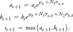
The option payoff P is then defined in the following equation:

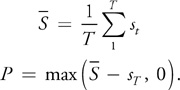
Figure 37-4 displays an example of the behavior of the correlated assets, and Listing 37-8 provides the code for a single path of the Asian basket simulation.

Figure 37-4 Example of One Run of the Asian Basket Simulation

Example 37-8. Code for a Single Path of the Asian Basket Simulation

    __device__ float AsianBasket(   unsigned T, float A_0, float B_0,   float MU_A, float SIG_AA,   float MU_B, float SIG_AB, float SIG_BB) {   float a=A_0, b=B_0, s=0, sum=0;   for(unsigned t=0;t<T;t++){     float ra=RNORM();     float rb=RNORM();     a*=exp(MU_A+ra*SIG_AA);     b*=exp(MU_B+ra*SIG_AB+rb*SIG_BB);     s=max(a,b);     sum+=s;   }   return max(sum/T-s,0); }

37.3.2 Variant on a Lookback Option

The second application is a variant on a lookback option (Wilmott 2006), with some special features. Specifically, the payoff is determined by the sum of the positive differences between the asset price at each time step, and the final asset price. This can be thought of as drawing a horizontal line across the asset path from the terminal price and using the area above the line and below the path as the payoff. Thus, if s ₀ . . . s_T is the path of the asset, the payoff P will be the following:

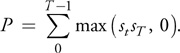
This option requires that the entire evolution of the path be stored, because the payoff can be determined only when the final price is known.

We also use a more complex type of asset price model in this option, called a GARCH model. This model incorporates the idea of time-varying volatility: basically, the idea that the size of the asset movement depends in part on the size of the most recent movement. This is often seen when a large change in a stock price is followed by another large change, while in more stable periods, the size of a change is lower. The asset path is modeled as follows:

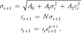
Figure 37-5 demonstrates the movement and relevant asset values, and Listing 37-9 provides the code for a single path of the lookback option simulation. When used in practice, the single-path functions shown in Listings 37-8 and 37-9 are called repeatedly such that results from a set of different simulation paths are combined into mean and variance results, as shown in Listing 37-10.

Figure 37-5 Movement of the Asset

Example 37-9. Code for a Single Path of the Lookback Option Simulation

    // (MAX_T%WARP_SIZE)==0    const unsigned MAX_T; __device__ float LookbackDiff(   unsigned T,   float VOL_0, float EPS_0,   float A_0, float A_1, float A_2   float MU ) {   __shared__ float path[NUM_THREADS*MAX_T];   float vol=VOL_0, eps=EPS_0;   float s=S0;   int base=__mul24(tid,MAX_T)-NUM_THREADS;   // Choose a random asset path.    for(unsigned t=0;t<T;t++){     // Store the current asset price.     base=base+NUM_THREADS;     path[base]=s;     // Calculate the next asset price.     vol=sqrt(A_0+A_1*vol*vol+A_2*eps*eps);     eps=RNORM()*vol;     s=s*exp(MU+eps);   }   // Look back at path to find payoff.    float sum=0;   for(unsigned t=0;t<T;t++){     base=base-NUM_THREADS;     sum+=max(path[base]-s,0);   }   return sum; }

Example 37-10. Making Use of the Individual Simulation Kernels

Results from the kernel runs are combined into mean and variance results, which can then be returned. We have left the parameters to SimKernel() vague here, to generalize over the two kernels described in Listings 37-8 and 37-9.

    // Extract a thread-specific seed from the array of seeds.    __device__ void InitRNORM(seeds); // Produce a random number from the thread's stream    // based on whichever generator we are using.    __device__ float RNORM(); // Execute the simulation kernel using calls to RNORM().    __device__ float SimKernel(parameters); __global__ float2 MonteCarloThread(seed, parameters) {   InitRNORM(seeds);   float mean=0, varAcc=0;   for(float i=1;i<=PATHS_PER_SIM;i++){     // Simulate one path.    float res=SimKernel(parameters);     // Now update mean and variance in    // numerically stable way.    float delta=res-mean;     mean+=delta/i;     varAcc+=delta*(res-mean);   }   float variance=S/(PATHS_PER_SIM-1);   return make_float2(mean,variance); }

37.3.3 Results

We have implemented the hybrid Tausworthe RNG with Box-Muller and the Wallace Gaussian RNG in CUDA and show the raw RNG performance results in the first column (labeled "Raw RNG") in Table 37-1. The results are measured in millions of Gaussian samples produced across the entire GPU every second (MSamples/s). The Wallace generator provides more than 5 billion samples per second, achieving a rate 1.2 times that of the hybrid Tausworthe generator. However, the Wallace transform also uses a large amount of shared memory to store the pool, in this case 2,048 words. This leaves only 2,048 words available to be used within simulation code; so in cases where simulations require all the shared memory, the slower Tausworthe generator must be used.

Table 37-1. Performance Results for the Discussed Random Number Generators and Simulations

The Constant RNG row represents the case where no real random numbers are being produced and the values are being taken directly from variables such that the simulation code is not optimized away. The Raw RNG column denotes the random number executing in isolation directly into memory with no simulation being driven.
		Raw RNG(MSamples/s)	Asian (MSteps/s)	Lookback(MSteps/s)
GPU	Tausworthe plus Box-Muller	4,327	1,769	1,147
Wallace	5,274	1,877	—
Constant RNG	—	5,177	2,908
Quad Opteron	Ziggurat plus Mersenne Twister	206	32	50
Constant RNG	—	44	64
	Speedup	26	59	23

Also included in the table are performance results for all four processors of a 2.2 GHz Quad Opteron, using a combination of the Mersenne twister uniform generator and Ziggurat transform. The GPU-based Wallace generator provides a speedup of 26 times over the quad-CPU machine, but this measures only raw RNG speed: it is also important to be able to do something with these random numbers.

Columns two and three of Table 37-1 show the performance of simulations for the two exotic options presented in the previous section. As well as the two GPU and one GPU based mentioned earlier, two further rows are included, both labeled "Constant RNG." In these cases the random number generator was removed, while taking care to ensure the rest of the simulation code is not optimized out, thus giving an idea of the ratio of time spent generating random numbers to time spent using them.

The performance figures are reported in MSteps/s, which is a measure of the number of simulation time steps that can be processed per second. For example, in the Asian option, each step corresponds to one iteration of the inner loop of Listing 37-8. When measuring the performance of the Asian option, each simulation executed 256 time steps, with 256 threads per block; so completing one block per second would provide 65 KSteps/s. In the lookback case, the number of time steps is limited by the amount of shared memory that can be dedicated to each thread. We used 512 threads per block; thus the lookback option was limited to 8 time steps per simulation.

In the Asian case, we see that the Wallace generator provides only a modest improvement of 1.06 times, compared to the Tausworthe/Box-Muller generators. The relative slowdown appears to be due to interactions between the Wallace code and simulation kernel code, possibly due to register allocation conflicts. Even so, the performance is 59 times that of the software implementation.

In the lookback case, the Wallace cannot be used because the shared memory is needed by the simulation kernel, and performance is much lower than that of the Asian option. Interestingly, the software implementation exhibits the opposite performance: the lookback is significantly faster than the Asian. However, a 23 times improvement in speed is seen by using the GPU rather than CPU-based solution.

37.4 Conclusion

Modern GPU hardware is highly capable of use in financial simulation. In this chapter, we have discussed approaches for generating random numbers for these kinds of simulation. Wallace's method provides good performance while maintaining a high quality of random numbers, as shown by statistical analysis. Due to resource limitations, tradeoffs are necessary, so the Wallace approach will not be the appropriate method to use in all situations. These trade offs should be manageable in most situations, and the use of CUDA and the GPU hardware for financial simulation should be a viable option in the future.

37.5 References

Brent, Richard P. 2003, "Some Comments on C. S. Wallace's Random Number Generators." The Computer Journal.

Colb, C., and M. Pharr. 2005. "Options Pricing on the GPU." In GPU Gems 2, edited by Matt Pharr, pp. 719–731. Addison-Wesley.

Knuth, D. 1969. The Art of Computer Programming, Volume 2: Seminumerical Algorithms. Addison-Wesley.

L'Ecuyer, P. 1996. "Maximally Equidistributed Combined Tausworthe Generators." Mathematics of Computation.

L'Ecuyer, P. 1999. "Tables of Maximally Equidistributed Combined LFSR Generators." Mathematics of Computation.

L'Ecuyer, P. 2006. "TestU01: A C Library for Empirical Testing of Random Number Generators." ACM Transactions on Mathematical Software.

Marsaglia, George. 1995. "The Diehard Battery of Tests of Randomness." http://www.stat.fsu.edu/pub/diehard/.

Marsaglia, George. 2000. "The Ziggurat Method for Generating Random Variables." Journal of Statistical Software.

Matsumoto, M. and T. Nishimura. 1998. "Mersenne Twister: A 623-Dimensionally Equidistributed Uniform Pseudorandom Number Generator." ACM Transactions on Modeling and Computer Simulation.

Metropolis, N. 1987. "The Beginning of the Monte Carlo Method." Los Alamos Science.

NVIDIA Corporation. 2007. NVIDIA CUDA Compute Unified Device Architecture Programming Guide. Version 0.8.1.

Press, W. H., S. A. Teukolsky, W. T. Vetterling, and B. P. Flannery. 1992. Numerical Recipes in C. Second edition. Cambridge University Press.

Sussman, M., W. Crutchfield, and M. Papakipos. 2006. "Pseudorandom Number Generation on the GPU." Graphics Hardware.

Wallace, C. S. 1996. "Fast Pseudorandom Generators for Normal and Exponential Variates." ACM Transactions on Mathematical Software.

Wilmott, P. 2006. Paul Wilmott on Quantitative Finance. Wiley.

Part II: Light and Shadows

Part III: Rendering

Part IV: Image Effects

Part V: Physics Simulation

Part VI: GPU Computing

Preface