This post is an update to an older post.
Deep learning models require training with vast amounts of data to achieve accurate results. Raw data usually cannot be directly fed into a neural network due to various reasons such as different storage formats, compression, data format and size, and limited amount of high-quality data.
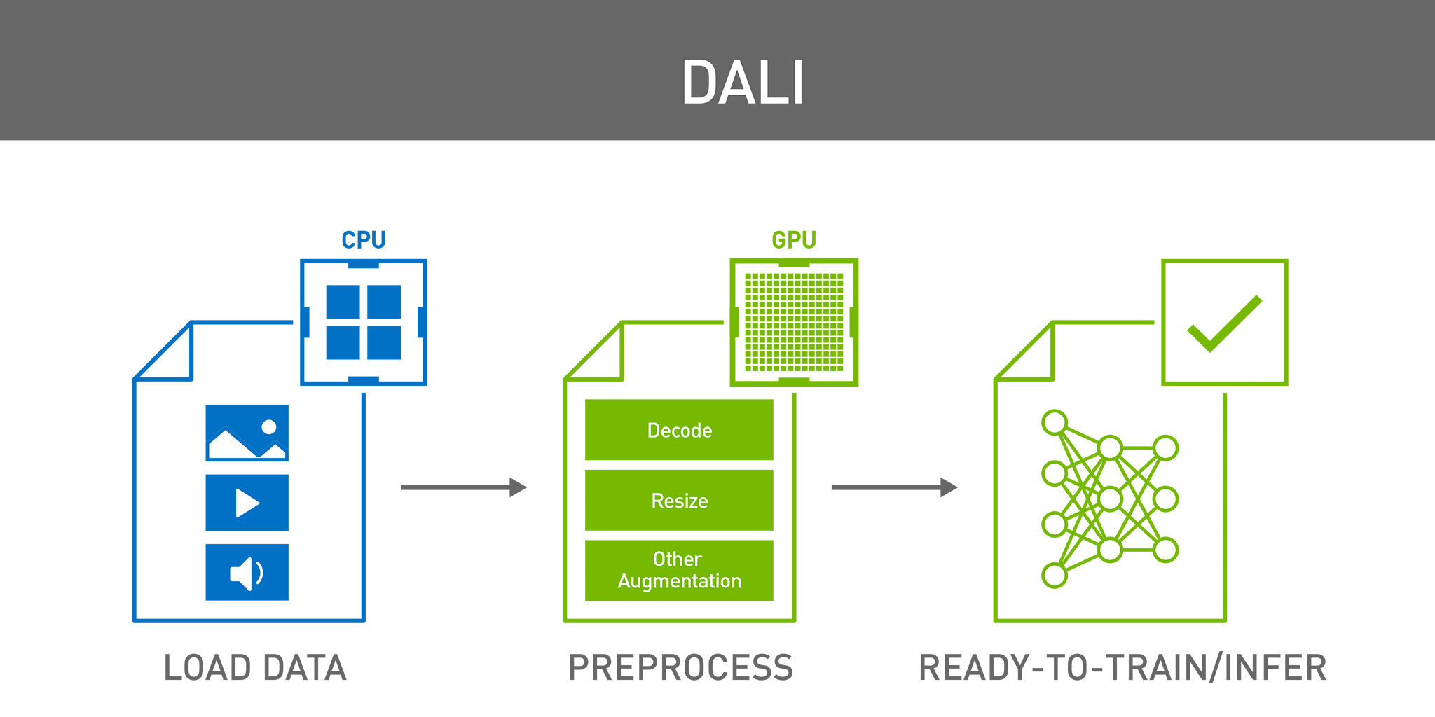
Addressing these issues requires extensive data preparation and preprocessing steps, from loading, decoding, decompression, to resizing, format conversion and various data augmentations.
Deep learning frameworks such as TensorFlow, PyTorch, MXNet, etc, offer native implementations for some of those preprocessing steps. This often brings portability issues, due to use of framework-specific data formats, availability of transformations, and implementation differences across frameworks.
The CPU bottleneck
Data preprocessing for deep learning workloads has garnered little attention until recently, eclipsed by the tremendous computational resources required for training complex models. As such, preprocessing tasks typically used to run on the CPU due to simplicity, flexibility, and availability of libraries such as OpenCV, Pillow or Librosa.
Recent advances in GPU architectures introduced in the NVIDIA Volta and NVIDIA Ampere Architectures, have significantly increased GPU throughput in deep learning tasks. In particular, half-precision arithmetic and Tensor Cores accelerate certain types of FP16 matrix calculations useful for training DNNs. Dense multi-GPU systems like the NVIDIA DGX-2 and DGX A100 train a model much faster than data can be provided by the input pipeline, leaving the GPUs starved for data.
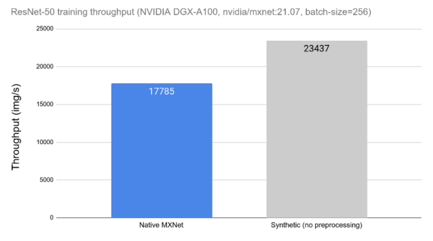
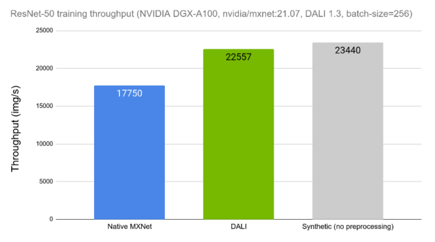
Today’s DL applications include complex, multi-stage data processing pipelines consisting of many serial operations. Relying on the CPU to handle these pipelines limits performance and scalability. In Figure 1, one can observe the impact of data preprocessing in the training throughput of a ResNet-50 network. On the left side we can see the throughput of the network when using the framework’s tools for data loading and preprocessing, which run on the CPU. On the right side, we can see the performance of the same network without the impact of data loading and preprocessing, by replacing it with synthetic data. This measurement can be used as a theoretical upper limit when comparing different data preprocessing tools.
DALI to the rescue
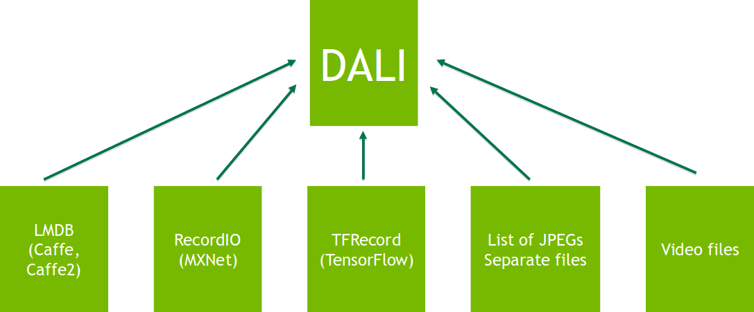
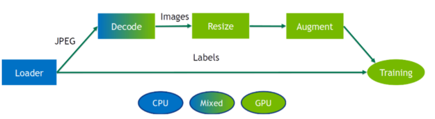
NVIDIA Data Loading Library (DALI) is a result of our efforts to find a scalable and portable solution to the data pipeline issues mentioned preceding. DALI is a set of highly optimized building blocks and an execution engine to accelerate input data pre-processing for Deep Learning (DL) applications (see Figure 2). DALI provides performance and flexibility for accelerating different data pipelines.
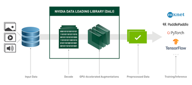
Figure 2: DALI overview and its usage as a tool for accelerated data loading and pre-processing in DL applications.
DALI offers data processing primitives for a variety of deep learning applications, such as classification or detection, and supports different data domains, including image, video, audio, and volumetric data.
The supported input formats include most commonly used image file formats (JPEG, PNG, TIFF, BMP, JPEG2000, NETPBM), NumPy arrays, video files encoded with many codecs (H.264, HEVC, VP8, VP9, MJPEG) as well as audio files (WAV, OGG, FLAC).
An important feature of DALI is plugins, which can be used as drop-in replacements for frameworks’ native datasets. Currently DALI comes with plug-ins for MXNet, PyTorch, TensorFlow, and PaddlePaddle. A DALI pipeline can be defined once and used with any of the supported frameworks by simply using a different data iterator wrapper.
On top of that, DALI natively supports different storage formats that are used in specific frameworks (e.g. LMDB in Caffe and Caffe2, RecordIO in MXNet, TFRecord in TensorFlow). This allows us to use any supported data format regardless of the DL framework being used. For example, we can use MXNet for the model, while keeping our data in TFRecord (the native TensorFlow data format).
DALI can be easily tailored for specific projects by configuring external data sources in Python, or extended with custom operators. Lastly, DALI is an open-source project, so you can readily extend it and adapt it to suit your particular needs.
DALI key concepts
The main entity in DALI is the data processing pipeline. A pipeline is defined by a symbolic graph of data nodes connected by operators. Each operator typically gets one or more inputs, applies some kind of data processing, and produces one or more outputs. There are special kinds of operators that don’t take any inputs and produce outputs. Those special operators act like a data source – readers, random number generators and external_source fall into this category. A pipeline definition is expressed in Python using imperative language, as in most of the current deep learning frameworks, but is run in an asynchronous fashion.
Once built, a pipeline instance can either be run explicitly by calling the pipeline’s run method, or wrapped with a data iterator specific to the target deep learning framework.
DALI offers CPU and GPU implementations for a wide range of processing operators. The availability of a CPU or GPU implementation depends on the nature of the operator. Make sure to check the documentation for an up-to-date list of supported operations, as it is expanded with every release.
DALI operators require the input data to be placed on the same device as the operator’s backend. Operators with a Mixed backend are a special kind that receives inputs placed on CPU memory and output data placed in GPU memory. For performance reasons, data transfer from GPU to CPU memory within a DALI pipeline is not accessible.
While most of DALI’s benefits are achieved when offloading processing to the GPU, sometimes it can be beneficial to keep part of the operations running on the CPU. Especially, in systems with a high CPU to GPU ratio, or in cases where the GPU is completely occupied with the model. The user can experiment with the CPU/GPU placement to find the sweet spot on a case-by-case basis.
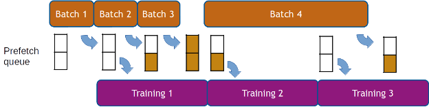
As stated earlier, DALI’s execution is asynchronous, which allows for data prefetching, that is, preparing batches of data ahead of time before they are requested so that the framework has always data ready for the next iteration. DALI handles data prefetching transparently for the user, with a configurable prefetch queue length. Data prefetching helps to hide the latency of preprocessing, which is important when the processing time varies significantly across iterations (see Figure 4).
How to use DALI
The easiest way to define a DALI pipeline is using the pipeline_def Python decorator. To create a pipeline we define a function where we instantiate and connect the desired operators, and return the relevant outputs. Then just decorate it with pipeline_def.
from nvidia.dali import pipeline_def, fn
@pipeline_def
def simple_pipeline():
    jpegs, labels = fn.readers.file(file_root=image_dir,
                                    random_shuffle=True,
                                    name="Reader")
    images = fn.decoders.image(jpegs)

    return images, labels
There are few things worth noting in this example pipeline. The first operator is a file reader that discovers and loads files contained in a directory. The reader outputs both the contents of the files (in this case, encoded JPEGs) and the labels, which are inferred from the directory structure. We’ve also enabled random shuffling and given a name to the reader instance, which will be important later when we integrate with the framework iterator. The second operator is an image decoder.
The next step is to instantiate a simple_pipeline object and build it to actually construct the graph. During pipeline instantiation, we are also defining the batch size, the number of CPU threads used for data processing, and the GPU device ordinal. For more options, refer to the documentation.
pipe = simple_pipeline(batch_size=32, num_threads=3, device_id=0)
pipe.build()
At this point, the pipeline is ready to use. We can obtain a batch of data by calling the run method.
images, labels = pipe.run()Now let us add some data augmentation, for example rotate each image by a random angle. To generate a random angle, we can use random.uniform, and rotate for the rotation:
@pipeline_def()
def rotate_pipeline():
    jpegs, labels = fn.readers.file(file_root=image_dir,
                                    random_shuffle=True,
                                    name="Reader")
    images = fn.decoders.image(jpegs)
    angle = fn.random.uniform(range=(-10.0, 10.0))
    rotated_images = fn.rotate(images, angle=angle, fill_value=0)
    return rotated_images, labels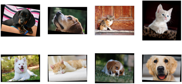
Figure 5: Example results of
rotate_pipeline. Each sample is rotated by a different angle.Offloading computation to the GPU
We can now modify our simple_pipeline so that it uses the GPU to perform augmentations. DALI makes this transition very easy. The only thing that changes is the definition of the rotate operator. We only need to set the device argument to “gpu” and make sure that its input is transferred to the GPU by calling .gpu().
self.rotate = fn.rotate(images.gpu(), angle=angle, device="gpu")To make things even simpler, we can even omit the device argument and let DALI infer the operator backed directly from the input placement.
self.rotate = fn.rotate(images.gpu(), angle=angle)That is it, simple_pipeline now performs the rotations on the GPU. Keep in mind that the resulting images are also allocated in the GPU memory, which is typically what we want, since the model requires the data in GPU memory. In any case, copying back the data to CPU memory after running the pipeline can be easily achieved by calling as_cpu on the objects returned by Pipeline.run.
images, labels = pipe.run()
images_host = images.as_cpu()
Frameworks integration
Seamless interoperability with different deep learning frameworks represents one of the best features of DALI. For example, to use your pipeline with a PyTorch model, we can easily do so by wrapping it with DALIClassificationIterator. For a more generic case, such as an arbitrary number of pipeline outputs, use DALIGenericIterator.
from nvidia.dali.plugin.pytorch import DALIGenericIterator
train_loader = DALIClassificationIterator([pipe], reader_name='Reader')
Note the argument reader_name, which value matches the name argument of the reader instance. The iterator will use that reader as a source of information for the number of samples in an epoch.
We can now enumerate the train_loader instance and feed the data batches to the model.
for i, data in enumerate(train_loader):
    images = data[0]["data"]
    target = data[0]["label"].squeeze(-1).long()
    # model training
More information about framework integration can be found in the framework plug-ins section of the documentation.
DALI in inference
Having equivalent definitions of the data processing steps for training and inference is crucial to achieve good accuracy results. Thanks to NVIDIA Triton Inference Server and its dedicated DALI backend, we can now easily deploy DALI pipelines to inference applications, making the data pipeline fully portable. In the architecture shown in Figure 6, a DALI pipeline is deployed as part of a TRITON ensemble model. This configuration has two main advantages. The first is that data processing is executed in the server, typically a more powerful machine than the client machine. The second benefit is that data can be sent to the server compressed, which saves network bandwidth.
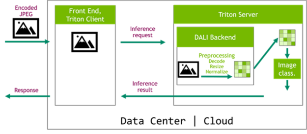
Make sure to check out our dedicated article Accelerating Inference with NVIDIA Triton Inference Server and NVIDIA DALI, covering this topic in more detail.
DALI’s impact in performance
NVIDIA showcases DALI in its implementations of SSD, ResNet-50, and RNN-T, being one of the contributing factors in our MLPerf benchmark success.
Let us compare the training throughput of a ResNet-50 network when using DALI compared to using the framework’s native solution. In Figure 7 we can see a similar comparison to the one presented in Figure 1, this time showing the results of using DALI for data loading and preprocessing as one of the options. We can see how the training throughput with DALI is much closer to the theoretical upper limit (synthetic example).
Now let us see how DALI affects the performance of Resnet50 inference in the Triton server. Figure 8 shows average inference request latency for offline preprocessing, meaning that the data was already preprocessed before starting the request, and online server-side preprocessing. The time spent is subdivided into communication overhead, data preprocessing and model inference. Due to the higher size of the decoded data, the latency of the preprocessed requests is severely affected by communication overhead. Because of that, the server-side preprocessing case is faster than the offline preprocessing case, even though the former includes data preprocessing time in the measurement.
![Bar chart with two groups of two bars. The vertical axis is labelled “Request latency [ms]” and the groups of bars are labelled as batch size 32 and 128, respectively. The bars in each group are labelled “No preprocessing” and “With DALI preprocessing”. The bars are divided in segments of different colors, used to denote the time spent in the following parts: Model inference time (yellow), preprocessing time (red), and communication overhead (blue).](https://developer-blogs.nvidia.com/wp-content/uploads/2021/10/RAPIDSData_Pic8-625x386.png)
Get started with DALI today
You can download the latest version of prebuilt and tested DALI pip packages. The NVIDIA GPU Cloud (NGC) Containers for TensorFlow, Pytorch, and MXNet have DALI integrated. You can review the many examples and read the latest release notes for a detailed list of new features and enhancements.
Triton DALI Backend is included in the Triton Inference Server container, starting from the 20.11 version.
See how DALI can help you accelerate data pre-processing for your deep learning applications. The best place to access is our documentation page, including numerous examples and tutorials. You can also watch our GTC 2021 talk about DALI. DALI is an open-source project, and our code is available on GitHub. We welcome your feedback and contributions.